Sage Journals: Discover world-class research

Abstract

Magnetic levitation planar motor has the characteristics of no friction loss, fast dynamic response, and real-time change of transportation track according to the demand. Therefore, a kind of magnetic levitation planar motor based on logistics transportation system is designed, which can meet the transportation needs of the logistics system through any combination of unit modules. Firstly, based on the mechanical model of magnetic levitation float in Halbach permanent magnet array magnetic field, establishing the thrust and torque model of maglev float. Secondly, according to the force/current relationship, considering the influence of uncertain parameters and load disturbance on the system, the decoupling control model of six degree of freedom motion system of magnetic levitation planar motor is established. Thirdly the adaptive contraction backstepping (ACB) controller is derived that can eliminate the uncertain disturbance of the nonlinear model and realize the real-time control of the system. The simulation and experimental results demonstrate that the method has expected response speed, strong robustness, and good dynamic tracking performance. Applying it to the logistics transportation system described in this article and has a good control effect.

Keywords

Magnetic levitation planar motor force/current model adaptive contraction backstepping control logistics transmission system

Introduction

Modern logistics plays a significant role in regional economic development. With the development of modernization and intelligent technology, the field of logistics transmission is changing. For example, the Production and Logistics Research Institute (BIBA) of the University of Bremen in Germany invented the modular universal cell conveyor belt “Celluveyor.” Its basic module was a logistics transmission unit composed of a regular hexagon, which could be combined arbitrarily according to the needs. The system controlled the rotation speed and direction of each module could transfer the goods according to the expected trajectory. However, Celluveyor has vibration problems when transporting goods, and cannot transport irregular or fragile items. Magnetic levitation planar motor (MLPM) has the advantages of no friction loss, fast dynamic response, and good stability.^1,2 Its combination has the characteristics of Celluveyor, faster speed, and lower energy consumption.³ It can transfer irregular or fragile items. In this device, each magnetic levitation planar motor is a unit module. Through the arbitrary combination of modules, it can realize the transportation requirements under different working conditions. This modular, decentralized integration new logistics system is the development direction of modern logistics transmission technology.

Applying MLPM in the field of logistics transportation has higher requirements for its control rapidity and stability. Lin designed the conventional PID control algorithm to the maglev control, the system response speed was not ideal, and the float could not achieve rapid levitation. Besides, the system had weak robustness. When the internal parameter perturbation or external interference, the system state would deviate from the equilibrium point.^4,5 Kou used ADRC to estimate the comprehensive disturbance of the system and compensate for the system in time. Compared with PID control, ADRC had good dynamic and robustness in a wide speed range.⁶ Huang et al.⁷ introduced the linearized feedback robust controller into the electromagnetic levitation system to ensure stability. However, the results showed that there were large overshoots and oscillations in the transient response of the system, which made it hard to implement in the real-time control of the magnetic levitation device.^8–11 Zhang linearized the maglev system at the equilibrium point. Designed an adaptive sliding mode controller with an integral sliding mode surface to realize the tracking of square wave and sine wave signal.^11,12

The above methods are hard to meet the requirements of dynamic and steady-state performance of the logistics transmission system under time-varying conditions. The backstepping design method¹³ is a method of system identification and model building, which has nice rapidity,^14,15 no overshoot under ideal conditions, and meets the requirements of system dynamics.^16–18 Besides, the integration of backstepping control and contraction control does not need to linearize the system at the equilibrium point, which is helping solve the modeling problem when the system parameters are not clear.

In this article, the thrust and torque model of the magnetic levitation planar motor is established to realize the decoupling of control variables with six degrees of freedom. Based on the force characteristics of the maglev float, the decoupling control model of the magnetic levitation planar motor is established considering the uncertain parameters of the model, and the external load disturbance. An adaptive contraction backstepping (ACB) controller for the MLPM decoupling model is designed. The method can realize the adaptive motion control of the magnetic levitation planar motor. The simulation results demonstrate that this method has expected response speed, strong robustness, and good dynamic tracking ability.

Structure and system modeling of magnetic levitation planar motor

Principle of magnetic levitation planar motor

The moving coil MLPM studied in this article consists of stator and float.¹⁹ The MLPM structure is shown in Figure 1. The float is a moving coil structure, which is composed of four coil groups.²⁰ The coil group consists of three coils. The two-dimensional Halbach permanent magnet array can provide three-dimensional distribution of the magnetic field. The two-dimensional Halbach magnetic array is composed of main magnetic steel and secondary magnetic steel.²¹ The main magnetic steel is square, and the secondary magnetic steel is rectangular.^22,23 The magnetization direction is parallel to the horizontal planar. The thickness of the main magnetic steel and the auxiliary magnetic steel is the same. The magnetization intensity is identical, and the magnetization is uniform.²⁴ The electrified coil in the magnetic field can generate both vertical and horizontal electromagnetic forces. Providing the levitation and driving force of the magnetic levitation planar motor.

Figure 1.

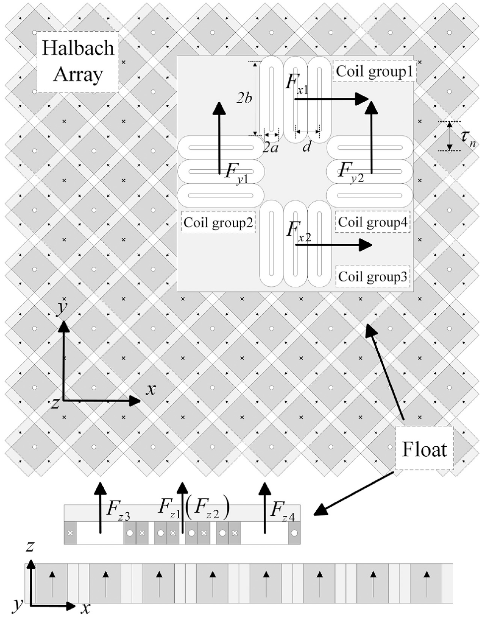
Structure of magnetic levitation planar motor.

In Figure 1, the width and length of coils are defined as 2a and 2b. The polar distance of the Halbach magnetic array is defined as $τ_{n}$ . The center distance of two adjacent coils in the coil group is defined as d. The group numbers of four coil groups are defined as 1, 2, 3, and 4 in the counter-clockwise order. The thrust generated by the coil group is defined as F_x₁, F_x₂, F_y₁, F_y₂, F_z₁, F_z₂, F_z₃, F_z₄.

Mathematical model of magnetic levitation planar motor

The mathematical model of MLPM is established by using the coil group as the basic driving unit. The spatial magnetic induction B of the Halbach permanent magnet array has the following distribution:

\begin{matrix} {[\begin{matrix} B_{x}, & B_{y}, & B_{z} \end{matrix}]}^{T} = B_{0} \exp (- \frac{π}{τ_{n}} z_{c}) \\ {[\begin{matrix} \sin (\frac{π}{τ_{n}} x_{c}), & \sin (\frac{π}{τ_{n}} y_{c}), & \cos (\frac{π}{τ_{n}} x_{c}) + \cos (\frac{π}{τ_{n}} y_{c}) \end{matrix}]}^{T} \end{matrix}

(1)

Where B_x, B_y, and B_z are the flux components along the three directions of x, y, and z. B₀ is the effective amplitude of the first harmonic of the flux density when z = 0, and $τ_{n}$ is half of the center distance between two adjacent magnets in the same direction, which is defined as the polar distance. Given the spatial distribution of magnetic induction and the shape and size of the coil, the thrust and torque are calculated by the Lorentz force formula²⁵

{\begin{matrix} F = \int_{V} J_{V} \times B dV \\ T = \int_{V} r \times J_{V} \times B dV \end{matrix}

(2)

Where J_V is the current density on the coil surface, B is the magnetic induction intensity, r is the arm of force corresponding to the volume element, and V is the coil volume. Taking coil group 1 as an example thrust on Halbach permanent magnet array can be described by equation (3)

\begin{matrix} [\begin{matrix} F_{x 1} \\ F_{y 1} \\ F_{z 1} \end{matrix}] = B_{0} \cdot \exp (- \frac{π}{τ_{n}} z_{c}) \cdot K_{Fx} \\ [\begin{matrix} \sin (\frac{π}{τ_{n}} x_{c} - d) & \sin (\frac{π}{τ_{n}} x_{c}) & \sin (\frac{π}{τ_{n}} x_{c} + d) \\ 0 & 0 & 0 \\ \cos (\frac{π}{τ_{n}} x_{c} - d) & \cos (\frac{π}{τ_{n}} x_{c}) & \cos (\frac{π}{τ_{n}} x_{c} + d) \end{matrix}] \cdot [\begin{matrix} J_{V 1} \\ J_{V 2} \\ J_{V 3} \end{matrix}] \end{matrix}

(3)

F_x ₁, F_y₁, and F_z₁ are the thrust of coil group 1, and K_Fx is the thrust influence coefficient considering the characteristics of coil diameter, thickness, and other factors, d is the center distance between two adjacent coils. The torque of the coil group in the Halbach permanent magnet array can be described as follows:

\begin{matrix} T_{x 1} = B_{0} \cdot \exp (- \frac{π}{τ_{n}} z_{c}) \cdot K_{Tx} \\ [\begin{matrix} \cos (\frac{π}{τ_{n}} x_{c} - d) & \cos (\frac{π}{τ_{n}} x_{c}) & \cos (\frac{π}{τ_{n}} x_{c} + d) \end{matrix}] [\begin{matrix} J_{V 1} \\ J_{V 2} \\ J_{V 3} \end{matrix}] \\ + \cos (\frac{π}{τ_{n}} y_{c}) (J_{V 1} + J_{V 2} + J_{V 3}) \end{matrix}

(4)

\begin{matrix} T_{y 1} = B_{0} \cdot \exp (- \frac{π}{τ_{n}} z_{c}) \cdot K_{Ta} \cdot K_{Tx} \\ [\begin{matrix} \sin (\frac{π}{τ_{n}} x_{c} - d) & \sin (\frac{π}{τ_{n}} x_{c}) & \sin (\frac{π}{τ_{n}} x_{c} + d) \end{matrix}] [\begin{matrix} J_{V 1} \\ J_{V 2} \\ J_{V 3} \end{matrix}] \\ + [\begin{matrix} \cos (\frac{π}{τ_{n}} x_{c} - d) & co s (\frac{π}{τ_{n}} x_{c}) & \cos (\frac{π}{τ_{n}} x_{c} + d) \end{matrix}] [\begin{matrix} J_{V 1} \\ J_{V 2} \\ J_{V 3} \end{matrix}] \end{matrix}

(5)

\begin{matrix} T_{z 1} = - B_{0} \cdot \exp (- \frac{π}{τ_{n}} z_{c}) \cdot K_{Tx} \\ [\begin{matrix} \sin (\frac{π}{τ_{n}} x_{c} - d) & \sin (\frac{π}{τ_{n}} x_{c}) & \sin (\frac{π}{τ_{n}} x_{c} + d) \end{matrix}] [\begin{matrix} J_{V 1} \\ J_{V 2} \\ J_{V 3} \end{matrix}] \end{matrix}

(6)

Where T_x₁, T_y₁, and T_z₁ are the torque of coil group 1, and K_Tx and K_Ta represent the torque influence coefficient considering the characteristics of coil diameter, thickness, and other factors.

Application of magnetic levitation planar motor in logistics transmission

Celluveyor has vibration during transportation and cannot transfer fragile goods. At the same time, the design of the conveyor belt makes it impossible to transport irregular shaped goods. MLPM has no appeal problem, and the block design enables it to transport irregular shaped goods through arbitrary combination behavior, as shown in Figure 2.

Figure 2.

Planar motor transport irregular and fragile goods.

The float driven by the current has a fast response speed. Through the reasonable distribution of force and current, each MLPM can realize 6-DOF motion. The upper computer takes MLPM as the smallest module, which can meet the requirements of high-precision transportation of modern logistics. Three MLPM cooperative movement as shown in Figure 3. Because MLPM is independent of each other, the next design takes one MLPM as the research object.

Figure 3.

Three MLPM cooperative movement.

Force/current model of magnetic levitation planar motor

As shown in Figure 1, coil groups 1 and 3 provide x-direction thrust components, coil groups 2 and 4 provide y-direction thrust components. All four coil groups can provide the z-axis vertical thrust components. The coil group of the float is taken as the driving unit, and the resultant force of z-axis is expressed as F_z = F_z₁ + F_z₂ + F_z₃ + F_z₄, the resultant force of the x-axis and y-axis is expressed as F_x = F_x₁ + F_x₂, F_y = F_y₁ + F_y₂, the coil torque is expressed as T_z = −l_x₁F_x₁ − l_y₂F_y₂ + l_x₃F_x₃ + l_y₄F_y₄, T_x = l_x₁F_x₁ + l_x₂F_x₂ − l_x₃F_x₃ − l_y₄F_y₄, T_y = −l_y₁F_y₁ + l_y₂F_y₂ +l_x₃F_x₃ − l_y₄F_y₄. Where F_x, F_y, F_z, T_x, T_y, T_z are the thrust and torque of the whole float, l_x, l_y represents the x-direction force arm and y-direction force arm from the action point of each thrust component to the mass center of the float.

After determining the thrust distribution method of the coil group, the current is applied to each coil to obtain the required thrust component. The current distribution method is related to two parameters, one is the number of coils in the coil group, which is defined as N, and the other is the center distance d of two adjacent coils in the coil group. The principle of the force/current model in the x-axis direction is the same as that in the y-axis direction. The electromagnetic force direction is different. Therefore, the x-axis is taken as an example for illustration.

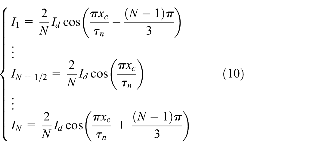
As shown in Figure 4, set the center position coordinate of the central coil in the coil group as (x_c, y_c, z_c), and use this to represent the position of the coil group in the global coordinate system. Coil group 1 with N coils, N is odd. The position coordinates of each coil in the coil group are (x_c, y_c, z_c), (x_c + d, y_c, z_c), and (x_c + (N − 1) d, y_c, z_c).

[\begin{matrix} F_{x 1} \\ F_{z 1} \end{matrix}] = B_{0} \cdot K_{Fx} \cdot \exp (- \frac{π}{τ_{n}} z_{c}) \cdot Q [\begin{matrix} I_{1} \\ ⋮ \\ I_{N + 1 / 2} \\ ⋮ \\ I_{N} \end{matrix}]

(7)

Where I₁, I₂, and I_N represent the current applied to the coil in the group, with the same amplitude. F_x₁ and F_z₁ are the thrust components of the x and z axes provided by the coil group. Q is a matrix.

{[\begin{matrix} \sin (\frac{π}{τ_{n}} x_{c} - \frac{(N - 1)}{3} d) & \cos (\frac{π}{τ_{n}} x_{c} - \frac{(N - 1)}{3} d) \\ \dots & \dots \\ \sin (\frac{π}{τ_{n}} x_{c}) & \cos (\frac{π}{τ_{n}} x_{c}) \\ \dots & \dots \\ \sin (\frac{π}{τ_{n}} x_{c} + \frac{(N - 1)}{3} d) & \cos (\frac{π}{τ_{n}} x_{c} + \frac{(N - 1)}{3} d) \end{matrix}]}^{T}

Figure 4.

Structure diagram of the coil group.

The equivalent current matrix required for thrust is as follows:

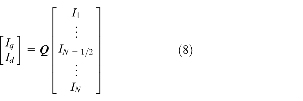
[\begin{matrix} I_{q} \\ I_{d} \end{matrix}] = Q [\begin{matrix} I_{1} \\ ⋮ \\ I_{N + 1 / 2} \\ ⋮ \\ I_{N} \end{matrix}]

(8)

I_q and I_d are the equivalent current required to provide horizontal thrust component and vertical thrust component. I_q is called quadrature axis current, and I_d is called direct axis current. Taking d as $4 τ_{n} / 3$ , the maximum thrust component provided by each coil group can be ensured when the three coils are orthogonal. Therefore, the current distribution is as follows, when coil group 1 generates thrust along the x horizontal direction.

{\begin{matrix} I_{1} = \frac{2}{N} I_{q} \sin (\frac{π x_{c}}{τ_{n}} - \frac{(N - 1) π}{3}) \\ ⋮ \\ I_{N + 1 / 2} = \frac{2}{N} I_{q} \sin (\frac{π x_{c}}{τ_{n}}) \\ ⋮ \\ I_{N} = \frac{2}{N} I_{q} \sin (\frac{π x_{c}}{τ_{n}} + \frac{(N - 1) π}{3}) \end{matrix}

(9)

Coil group 1 produces a horizontal thrust F_x₁ along the x-axis. The torque T_y₁ around the y-axis and T_z₁ around the z-axis generated by distributed force on coil group 1 are not zero. When coil group 1 produces levitation force along the z-axis

{\begin{matrix} I_{1} = \frac{2}{N} I_{d} \cos (\frac{π x_{c}}{τ_{n}} - \frac{(N - 1) π}{3}) \\ ⋮ \\ I_{N + 1 / 2} = \frac{2}{N} I_{d} \cos (\frac{π x_{c}}{τ_{n}}) \\ ⋮ \\ I_{N} = \frac{2}{N} I_{d} \cos (\frac{π x_{c}}{τ_{n}} + \frac{(N - 1) π}{3}) \end{matrix}

(10)

Then the levitation force F_z₁ in the vertical direction along the z-axis produced by coil group 1. The torque T_x₁ around the x-axis and the torque T_y₁ around the y-axis generated by the distributed force on coil group 1 are not zero.

Besides, if the horizontal thrust of coil groups 1 and 3 along the x and y axes are equal and opposite, they cancel each other. The torque around the x-axis and y-axis produced by the two groups of coils is zero, and the torque around the z-axis is the same and overlapped. At this time, the torque around the z-axis produced by two groups of coils is zero, and the torque around the y-axis and z-axis is zero by making the levitation force of coil groups 1 and 3 equal in the vertical direction of the y-axis and z-axis. The torque around the x-axis is the same and overlapped with each other. The float produces the torque around the x-axis.

Adaptive contraction backstepping control of magnetic levitation planar motor

Dynamic model of magnetic levitation planar motor

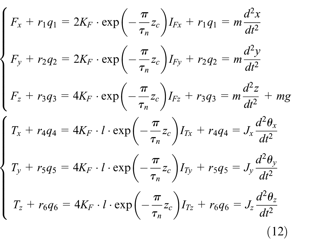
In addition to gravity, the force exerted on MLPM float includes the electromagnetic force between the permanent magnet array and the floating coil. The rigid disturbance is attributed to the load change, and the flexible perturbation is reduced to the damping term. The motion controller can suppress the disturbance force. In the process of establishing the MLPM dynamic model, the influence of gravity, and electromagnetic force on the system is considered. The dynamic model is

\begin{matrix} [\begin{matrix} F_{x} \\ F_{y} \\ F_{z} \\ T_{x} \\ T_{y} \\ T_{z} \end{matrix}] = [\begin{matrix} m \\ m \\ m \\ J_{x} \\ J_{y} \\ J_{z} \end{matrix}] [\begin{matrix} \overset{\cdot\cdot}{x} \\ \overset{\cdot\cdot}{y} \\ \overset{\cdot\cdot}{z} \\ {\overset{\cdot\cdot}{θ}}_{x} \\ {\overset{\cdot\cdot}{θ}}_{y} \\ {\overset{\cdot\cdot}{θ}}_{z} \end{matrix}] \\ + [\begin{matrix} 0 \\ 0 \\ mg \\ 0 \\ 0 \\ 0 \end{matrix}] + [\begin{matrix} h_{x} \\ h_{y} \\ h_{z} \\ h_{tx} \\ h_{ty} \\ h_{tz} \end{matrix}] \end{matrix}

(11)

Where F_x, F_y, F_z, T_x, T_y, and T_z represent thrust and electromagnetic torque, h_x, h_y, h_z, h_tx, h_ty, and h_tz represent the load force generated by rigid disturbance, m represents the mass of the float. J_x, J_y, and J_z represents the moment of inertia of the float around each rotation axis. x, y, z represents the translational displacement of the float in all directions. $θ_{x}$ , $θ_{y}$ , $θ_{z}$ represents the angular displacement of the float around each axis, and g is the acceleration of gravity.

Based on the dynamic model and formulae (3)–(6) of MLPM, establish the equation of the magnetic levitation planar motor.

\begin{matrix} {\begin{matrix} F_{x} + r_{1} q_{1} = 2 K_{F} \cdot \exp (- \frac{π}{τ_{n}} z_{c}) I_{Fx} + r_{1} q_{1} = m \frac{d^{2} x}{d t^{2}} \\ F_{y} + r_{2} q_{2} = 2 K_{F} \cdot \exp (- \frac{π}{τ_{n}} z_{c}) I_{Fy} + r_{2} q_{2} = m \frac{d^{2} y}{d t^{2}} \\ F_{z} + r_{3} q_{3} = 4 K_{F} \cdot \exp (- \frac{π}{τ_{n}} z_{c}) I_{Fz} + r_{3} q_{3} = m \frac{d^{2} z}{d t^{2}} + mg \end{matrix} \\ {\begin{matrix} T_{x} + r_{4} q_{4} = 4 K_{F} \cdot l \cdot \exp (- \frac{π}{τ_{n}} z_{c}) I_{Tx} + r_{4} q_{4} = J_{x} \frac{d^{2} θ_{x}}{d t^{2}} \\ T_{y} + r_{5} q_{5} = 4 K_{F} \cdot l \cdot \exp (- \frac{π}{τ_{n}} z_{c}) I_{Ty} + r_{5} q_{5} = J_{y} \frac{d^{2} θ_{y}}{d t^{2}} \\ T_{z} + r_{6} q_{6} = 4 K_{F} \cdot l \cdot \exp (- \frac{π}{τ_{n}} z_{c}) I_{Tz} + r_{6} q_{6} = J_{z} \frac{d^{2} θ_{z}}{d t^{2}} \end{matrix} \end{matrix}

(12)

Where $K_{F} = K_{Fx} \cdot B_{0}$ is the product of the long side thrust coefficient of the coil and the magnetic induction intensity distribution amplitude B₀ on the surface of the permanent magnet array, and z_c is the air gap height of the MLPM float, that is, the vertical displacement. I_Fx, I_Fy, I_Fz, I_Tx, I_Ty, and I_Tz are the control currents output by the vertical motion controller in all directions, which are determined by the position servo control algorithm. The decoupling relationship between them and I_q, I_d is given in Sun et al.²⁵ l is the length of the coil. Apply the direct axis and quadrature axis current to each coil. $r_{1} q_{1}$ , $r_{2} q_{2}$ , $r_{3} q_{3}$ , $r_{4} q_{4}$ , $r_{5} q_{5}$ , $r_{6} q_{6}$ is a disturbance term and an uncertain parameter. The motion of six degrees of freedom of the magnetic levitation MLPM system.

Design of adaptive contraction backstepping controller for MLPM

Basic principle of contraction theory

Consider the smooth nonlinear system as

\overset{\cdot}{x} = f (x, t)

(13)

The exponential convergence of the trajectory of state x with time can be analyzed by virtual displacement.²⁶ The virtual displacement represents the linear minuteness increment between two points at the same time in space, denoted as $δ x$ . The virtual displacement is introduced into equation (13), that is,

δ \overset{\cdot}{x} = δ f = δ f / δ x \cdot (x, t) δ x

(14)

Perform the state-dependent coordinate transformation in equation (14),

δ z = Ω (x, t) δ x

(15)

Where $Ω (x, t)$ is the uniformly inverse matrix, and the metric uniformly symmetric positive definite matrix $P = Ω^{T} Ω$ representing Riemannian space is defined. Then, from the knowledge of differential geometry, the transformed trajectory square distance is

δ z^{T} δ z = δ x^{T} P δ x

(16)

The rate of change of the distance over time can be expressed as

d / dt \cdot δ z^{T} δ z = 2 δ z^{T} F δ z

(17)

Where $F = (\overset{\cdot}{Ω} + Ω \frac{\partial f}{\partial x}) Ω^{- 1}$ , then $d (δ z^{T} δ z) / dt \leq 2 λ_{max} δ z^{T} δ z$ , $λ_{max}$ is the largest eigenvalue of matrix F , and the inequality can be obtained

‖ δ z ‖ \leq ‖ δ z_{0} ‖ e^{\int_{0}^{t} λ_{max} dt}

(18)

Where $δ z_{0}$ is the virtual displacement of the initial state. $λ_{max}$ is uniformly strictly negative definite. There is a matrix measure $μ$ , $a > 0$ , such that $μ (f) \leq - a$ , then $δ z$ exponent converges to 0, and a is the contraction rate.

The matrix measure to determine the contraction of the system is $μ (F) = λ_{max} (F + F^{T}) / 2$ . If equation (13) is bounded by disturbance $ε (x, t)$ , then the distance is defined as the trajectory accords with equation (13), which meets the equation

\overset{\cdot}{x} = f (x, t) + ε (x, t)

(19)

If we define the distance $R = \int_{p_{1}}^{p_{2}} ‖ δ x^{T} p δ x ‖$ , $P_{1}$ as the locus meet formula (1) and $P_{2}$ as the locus meet formula (13), then we can prove that²⁷

R + | λ_{max} | R \leq ‖ Ω ε ‖

(20)

In the contraction analysis of the second-order closed-loop system, the fictitious displacement with layered connection can be expressed by equation (8). When $J_{11}$ , $J_{22}$ is negative definite and $J_{12}$ is smooth and bounded, the whole system is contracting, that is,

\frac{d}{dt} [\begin{matrix} δ z_{1} \\ δ z_{2} \end{matrix}] = [\begin{matrix} J_{11} & J_{12} \\ 0 & J_{22} \end{matrix}] [\begin{matrix} δ z_{1} \\ δ z_{2} \end{matrix}]

(21)

The control of x, y, z axes, and $θ_{x}$ , $θ_{y}$ , $θ_{Z}$ of MLPM are decoupled. Take the z-axis as an example for backstepping design. The basic idea is to select appropriate state variables from the original system and decompose them into new subsystems. Then virtual control law is designed for each subsystem. Finally, the actual control law of the system is obtained, which makes the whole system achieve the desired performance.²⁸

Design of contraction backstepping controller

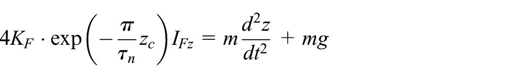
According to the dynamic equation of z-axis in formula (12)

4 K_{F} \cdot \exp (- \frac{π}{τ_{n}} z_{c}) I_{Fz} = m \frac{d^{2} z}{d t^{2}} + mg

Define the state variable as $x_{1} = z$ , $x_{2} = \overset{\cdot}{z}$ . The control quantity is defined as $u = I_{Fz}$ , consider the second-order dynamic equation as

{\begin{matrix} {\overset{\cdot}{x}}_{1} = x_{2} \\ {\overset{\cdot}{x}}_{2} = c η \cdot u - ρ \end{matrix}

(22)

Where $c$ is the coefficient $4 K_{F} / m$ , $η$ is $\exp (- π \cdot z_{c} / τ_{n})$ concerning the z-axis height, u is the controller input, and $ρ$ is the general constant g.

(1) The tracking error is defined as $e = x_{1} - x_{1}^{*}$ , $x_{1}^{*}$ is the reference position, let $x_{2} = x_{s} + β (x_{1})$ . Define the auxiliary variable as $x_{s} = x_{2} - β (x_{1})$ can be regarded as the error reference value of subsystem. Where $x_{1}^{*}$ is smooth and bounded, $β (x_{1})$ is the virtual control input. Therefore, formula (22) can be rewritten as

{\begin{matrix} {\overset{\cdot}{x}}_{1} = x_{s} + β (x_{1}) \\ {\overset{\cdot}{x}}_{2} = c η \cdot u - ρ \end{matrix}

(23)

The exponential convergence of the trajectory of state x₁ with time is analyzed by virtual displacement. The virtual displacement represents the linear minuteness increment between two points at the same time in space, denoted as $δ x_{1}$ . Introduce the virtual displacement into equation (23).

δ {\overset{\cdot}{x}}_{1} = δ x_{s} + J_{11} δ x_{1}

(24)

The Jacobian matrix can be expressed as

J_{11} = \frac{\partial [β (x_{1})]}{\partial x_{1}}

(25)

To make the first subsystem contract to x₁, that is, the Jacobian matrix $J_{11}$ is uniformly negative definite, $J = {\overset{\cdot}{J}}_{11} \leq - a_{1} < 0$ is established, where a₁ is a positive number, which is called contraction rate. The virtual control variable $β (x_{1})$ can be designed as

β (x_{1}) = {\overset{\cdot}{x}}_{1}^{*} - k_{1} (x_{1} - x_{1}^{*}) = {\overset{\cdot}{x}}_{1}^{*} - k_{1} e

(26)

Therefore, the differential form of tracking error can be written as

\overset{\cdot}{e} = {\overset{\cdot}{x}}_{1} - {\overset{\cdot}{x}}_{1}^{*} = x_{2} - {\overset{\cdot}{x}}_{1}^{*} = - k_{1} e + x_{s}

(27)

(2) After deriving the auxiliary variable x_s, get the formulae (25) and (26)

\begin{matrix} {\overset{\cdot}{x}}_{s} = {\overset{\cdot}{x}}_{2} + k_{1} \overset{\cdot}{e} - {\overset{\cdot\cdot}{x}}_{1}^{*} \\ = c η \cdot u - ρ + k_{1} ({\overset{\cdot}{x}}_{1} - {\overset{\cdot}{x}}_{1}^{*}) - {\overset{\cdot\cdot}{x}}_{1}^{*} \\ = \frac{4 K_{F}}{m} e^{(- \frac{π}{τ_{n}} z_{c})} \cdot I_{Fz} - g + k_{1} ({\overset{\cdot}{x}}_{1} - {\overset{\cdot}{x}}_{1}^{*}) - {\overset{\cdot\cdot}{x}}_{1}^{*} \end{matrix}

(28)

For the contraction backstepping control system, the virtual displacement state-space form of equations (27) and (28) can be expressed as

[\begin{matrix} δ \overset{\cdot}{e} \\ δ {\overset{\cdot}{x}}_{s} \end{matrix}] = [\begin{matrix} J_{11} & J_{12} \\ J_{21} & J_{22} \end{matrix}] [\begin{matrix} δ e \\ δ x_{s} \end{matrix}]

(29)

Let Jacobian matrix $J = [\begin{matrix} J_{11} & J_{12} \\ J_{21} & J_{22} \end{matrix}]$ . It is necessary to prove that the system meets the contraction criterion $μ (J) \leq - a$ . The system is exponentially stable if it can form the hierarchical connection. Where

\begin{matrix} J_{11} = \frac{\partial (- k_{1} e + x_{s})}{\partial e}, J_{12} = \frac{\partial (- k_{1} e + x_{s})}{\partial x_{s}}, \\ J_{21} = \frac{\partial (4 \frac{K_{F}}{m} e^{(- \frac{π}{τ_{n}} z_{c})} \cdot I_{Fz} - g - {k_{1}}^{2} e + k_{1} x_{s} - {\overset{\cdot\cdot}{x}}_{1}^{*})}{\partial e}, \\ J_{22} = \frac{\partial (4 \frac{K_{F}}{m} e^{(- \frac{π}{τ_{n}} z_{c})} \cdot I_{Fz} - g - {k_{1}}^{2} e + k_{1} x_{s} - {\overset{\cdot\cdot}{x}}_{1}^{*})}{\partial x_{s}} . \end{matrix}

(3) To ensure that x_s can contract, the actual control value u can be designed as follows:

\begin{matrix} u = \frac{[- k_{2} x_{s} + ρ - k_{1} ({\overset{\cdot}{x}}_{1} - {\overset{\cdot}{x}}_{1}^{*}) + {\overset{\cdot\cdot}{x}}_{1}^{*}]}{c η} \\ = \frac{[- k_{2} x_{s} + g - k_{1} ({\overset{\cdot}{x}}_{1} - {\overset{\cdot}{x}}_{1}^{*}) + {\overset{\cdot\cdot}{x}}_{1}^{*}]}{\frac{4 K_{F}}{m} e^{(- \frac{π}{τ_{n}} z_{c})}} \end{matrix}

(30)

The control variable u is brought into (27) to make the eigenvalue $λ_{max}$ of the matrix negative definite by adjusting the parameters, $μ (J) \leq - a < 0$ . Therefore, equation (30) is incrementally stable. The system contracts to the desired trajectory.

Design of adaptive contraction backstepping controller

In practical application, should not ignore the load disturbance and the uncertain parameters of the magnetic levitation planar motor. Therefore, it is classified as a disturbance term. The adaptive term is added to the control rate to eliminate it.

(1) Consider the dynamic model with disturbance and uncertain parameters

{\begin{matrix} {\overset{\cdot}{x}}_{1} = x_{2} \\ {\overset{\cdot}{x}}_{2} = c η \cdot u - ρ + rq \end{matrix}

(31)

Where r is an uncertain parameter and q is a smooth bounded function.

(2) Consider that x_t is the actual error value including uncertain parameters, expressed as

\begin{matrix} {\overset{\cdot}{x}}_{t} = {\overset{\cdot}{x}}_{2} + k_{1} \overset{\cdot}{e} - {\overset{\cdot\cdot}{x}}_{1}^{*} \\ = c η \cdot u - ρ + k_{1} ({\overset{\cdot}{x}}_{1} - {\overset{\cdot}{x}}_{1}^{*}) - {\overset{\cdot\cdot}{x}}_{1}^{*} + rq \\ = \frac{4 K_{F}}{m} e^{(- \frac{π}{τ_{n}} z_{c})} \cdot I_{Fz} - g + k_{1} ({\overset{\cdot}{x}}_{1} - {\overset{\cdot}{x}}_{1}^{*}) - {\overset{\cdot\cdot}{x}}_{1}^{*} + rq \end{matrix}

(32)

(3) Based on the contraction backstepping (CB) method, an adaptive controller is designed

\begin{matrix} u = \frac{[- k_{2} x_{t} + ρ - k_{1} ({\dot{x}}_{1} - {\dot{x}}_{1}^{*}) + {\overset{\cdot\cdot}{x}}_{1}^{*} - \overset{⌢}{r} q]}{c η} \\ = \frac{[- k_{2} x_{t} + g - k_{1} ({\dot{x}}_{1} - {\dot{x}}_{1}^{*}) + {\overset{\cdot\cdot}{x}}_{1}^{*} - \overset{⌢}{r} q]}{\frac{4 K_{F}}{m} e^{(- \frac{π}{τ_{n}} z_{c})}} \end{matrix}

(33)

Where $\overset{⌢}{r}$ is the estimated value of the uncertain parameter, and its update rate can be defined as

\dot{\overset{⌢}{r}} = q^{T} (x_{t} - x_{s}) = q^{T} x_{t}

(34)

Where x_s is considered to be the error reference value close to 0, so there is $q^{T} (x_{t} - x_{s}) = q^{T} x_{t}$ . If $x_{s} = 0$ , the adaptive system can be constructed as

[\begin{matrix} δ {\overset{\cdot}{x}}_{t} \\ δ \overset{\cdot}{\tilde{γ}} \end{matrix}] = [\begin{matrix} \frac{\partial f (x_{1}, t)}{\partial z_{1}} & q \\ - q^{T} & 0 \end{matrix}] [\begin{matrix} δ x_{t} \\ δ \tilde{γ} \end{matrix}]

(35)

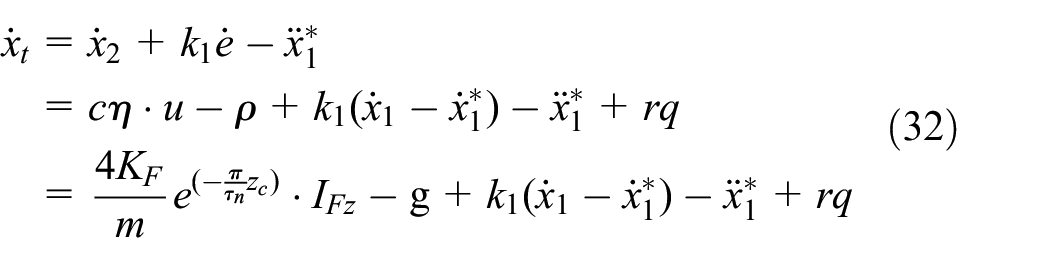
Therefore, $\partial f (x_{t}, t) / \partial x_{t} = - k_{2}$ can be contracted by adjusting the parameters, $x_{t}$ -exponent converges to 0, and $γ$ is bounded. So, the control system is stable. And by selecting $k_{1}$ , $k_{2}$ , the system can obtain better rapidity and stability.

Finally, the MLPM system model with uncertain parameters derived from the z-axis is

{\begin{matrix} {\overset{\cdot}{x}}_{1} = x_{2} \\ {\overset{\cdot}{x}}_{2} = c η \cdot u - ρ + rq \end{matrix}

(36)

The state variable is extended to the input control of x, y, z, axes, and $θ_{x}$ , $θ_{y}$ , $θ_{Z}$ ,²⁹ so that

\begin{matrix} {[x_{1}, x_{2}, x_{3}, x_{4}, x_{5}, x_{6}]}^{T} = [x, y, z, θ_{x}, θ_{y}, θ_{z}]^{T} \\ {[x_{7}, x_{8}, x_{9}, x_{10}, x_{11}, x_{12}]}^{T} = [\overset{\cdot}{x}, \overset{\cdot}{y}, \overset{\cdot}{z}, {\overset{\cdot}{θ}}_{x}, {\overset{\cdot}{θ}}_{y}, {\overset{\cdot}{θ}}_{z}]^{T} \end{matrix}

Define the control quantity as

u = {[\begin{matrix} I_{Fx}, & I_{Fy}, & I_{Fz}, & I_{Tx}, & I_{Ty}, & I_{Tz}, \end{matrix}]}^{T},

Uncertain parameters are updated to

rq = {[\begin{matrix} \begin{matrix} r_{1} q_{1}, & r_{2} q_{2} \end{matrix}, & r_{3} q_{3}, & r_{4} q_{4}, & r_{5} q_{5}, r_{6} q_{6} \end{matrix}]}^{T}

Finally, as shown in Figure 5, considering the nonlinear motion model of magnetic levitation planar motor with uncertain parameters applied to logistics devices, the adaptive contraction backstepping (ACB) controller designed in this article can be described as follows:

\begin{matrix} c_{1} η_{1} = 1 / \frac{2 K_{F}}{m} e^{(- \frac{π}{τ_{n}} z_{c})}, c_{2} η_{2} = 1 / \frac{2 K_{F}}{m} e^{(- \frac{π}{τ_{n}} z_{c})}, \\ c_{3} η_{3} = 1 / \frac{4 K_{F}}{m} e^{(- \frac{π}{τ_{n}} z_{c})}, c_{4} η_{4} = 1 / \frac{4 K_{F} l}{J_{x}} e^{(- \frac{π}{τ_{n}} z_{c})}, \\ c_{5} η_{5} = 1 / \frac{4 K_{F} l}{J_{y}} e^{(- \frac{π}{τ_{n}} z_{c})}, c_{6} η_{6} = 1 / \frac{4 K_{F} l}{J_{z}} e^{(- \frac{π}{τ_{n}} z_{c})} . \end{matrix}

\begin{array}{l} [\begin{matrix} I_{F x} \\ I_{F y} \\ I_{F z} \\ I_{T x} \\ I_{T y} \\ I_{T z} \end{matrix}] = [\begin{matrix} c_{1} η_{1} \\ c_{2} η_{2} \\ c_{3} η_{3} \\ c_{4} η_{4} \\ c_{5} η_{5} \\ c_{6} η_{6} \end{matrix}] \cdot \\ ([\begin{matrix} - k_{2} x_{t 1} - k_{1} (x_{1} - x_{1}^{*}) + {\overset{\cdot\cdot}{x}}_{1}^{*} \\ - k_{4} x_{t 2} - k_{3} (x_{2} - x_{2}^{*}) + {\overset{\cdot\cdot}{x}}_{2}^{*} \\ - k_{6} x_{t 3} - k_{5} (x_{3} - x_{3}^{*}) + {\overset{\cdot\cdot}{x}}_{3}^{*} + g \\ - k_{8} x_{t 4} - k_{7} (x_{4} - x_{4}^{*}) + {\overset{\cdot\cdot}{x}}_{4}^{*} \\ - k_{10} x_{t 5} - k_{9} (x_{5} - x_{5}^{*}) + {\overset{\cdot\cdot}{x}}_{5}^{*} \\ - k_{12} x_{t 6} - k_{11} (x_{6} - x_{6}^{*}) + {\overset{\cdot\cdot}{x}}_{6}^{*} \end{matrix}] - [\begin{matrix} {\overset{⌢}{r}}_{1} q_{1} \\ {\overset{⌢}{r}}_{2} q_{2} \\ {\overset{⌢}{r}}_{3} q_{3} \\ {\overset{⌢}{r}}_{4} q_{4} \\ {\overset{⌢}{r}}_{5} q_{5} \\ {\overset{⌢}{r}}_{6} q_{6} \end{matrix}]) \end{array}

(37)

Figure 5.

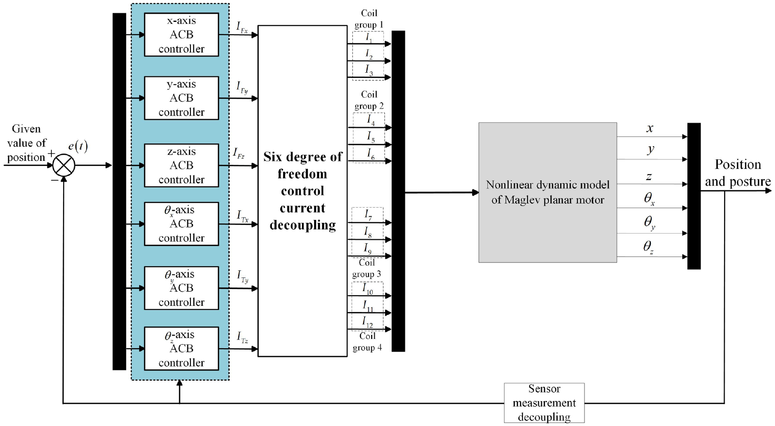
Decoupling block diagram of 6-DOF planar motor control.

Experimental verification

The correctness of the adaptive contraction backstepping controller is verified on the MATLAB software experimental platform. Simulate the start-up process, the initial state of the z-axis is set to 0, and the z-axis stable height is set to a fixed height of 5 mm. For the expected trajectory of the x-axis and rotation angle, due to the similarity of control, the horizontal motion and angular motion of the x-axis are carried out verification.³⁰ Figure 5 shows the z-direction closed-loop control model of MLPM.

The simulation experiment of the planar motor is shown in Figure 6. The parameters of the experimental platform are shown in Table 1.

Figure 6.

Magnetic levitation control system based on adaptive contraction backstepping controller.

Table 1.

Parameters of magnetic levitation planar motor.

Physical parameters	Value
Float mass, m/kg	1.2
Moment of inertia, J/kg m²	1.67 × 10⁻³
Number of turns, n	54
Gravitational acceleration, g/m/s²	9.8
K_Fx thrust coefficient, m	6.04 × 10⁻²

As shown in Figure 7 that when MLPM model parameters are uncertain, the stability time of traditional PID is 0.0043 s and the overshoot reaches 24%. The stability time of the ACB controller is 0.0025 s, which finally stabilizes at 5 mm without static error and overshoot. When 0.025 s, the system is subject to 10% external disturbance, and the fluctuation is 1 mm. The traditional PID controller is stable after 0.002 s, while the ACB controller is 0.0015 s stable, and its control performance is close to the ideal backstepping control.

Figure 7.

(a) PID control z-axis height and (b) ACB control z-axis height.

Therefore, when the ACB control algorithm is used, MLPM can start quickly, track the desired trajectory state, and the change is kept in a small range. When the disturbance occurs in 0.025 s, the system has good anti disturbance ability. But the PID control algorithm has a general effect, with certain overshoot and response speed has a gap with ACB algorithm.

As shown in Figure 2, each MLPM can be suspended at a specific height when the logistics transmission system designed in this paper is used to lift the goods. The levitation height of MLPM1 is 6 mm, that of MLPM2 is 8 mm, and that of MLPM3 is 7 mm. The lifting time is 0.025 s. This working model can transport fragile and irregular shaped goods. It can be seen from the simulation Figure 8 that compared with the PID controller, the response speed under ACB control is fast, and the vibration suppression effect is good.

Figure 8.

(a) PID controls three MLPM to lift irregular shaped goods and (b) ACB controls three MLPM to lift irregular shaped goods.

According to the comparison in Figure 9, the overshoot of the traditional PID controller for x-axis displacement and rotation radian is 25% and 28%, and the stabilization time is 0.0035 and 0.004 s. The stability time of the ACB controller is 0.002 and 0.018 s. Finally, it is stabilized at 5 mm and 1.5 mrad. At 0.015 s, adding the sine wave disturbance with the amplitude of 10% for 0.02 s, it can be seen that ACB in Figure 8 has a better suppression effect. ACB controller has better tracking performance, which can make the x-axis trajectory follow the desired trajectory. Its control performance is close to the ideal backstepping control and retains the nonlinearity of the system. The adaptive term has a good suppression effect on the uncertain parameters of the system. The tracking performance of traditional PID control is not as good as the ACB designed in this article, and its stability is poor.

Figure 9.

(a) x-Axis displacement and x-axis displacement disturbance suppression and (b) x-axis angular motion and x-axis deflection disturbance suppression.

In the simulation environment, verify the preset trajectory output performance of the magnetic levitation planar motor system. The float motion trajectory in the three-dimensional space is shown in Figure 10. The preset trajectory in (a) is circular. It can be seen from (a) that ACB control has an excellent trajectory output effect on circular trajectory. The preset trajectory in (b) is a regular hexagon. It can be seen from (b) that the ACB control effect is still good.

Figure 10.

(a) Three-dimensional trajectory of circular motion and (b) three-dimensional trajectory of hexagon motion.

As shown in Figure 11, a high-precision MEMS sensor is installed on the float to measure its actual motion trajectory. In the experimental platform, MPU9250, 16-bit data precision is used to collect the acceleration data of the x-axis and y-axis in real-time. Then the data is filtered and converted into displacement and fed back to the oscilloscope.

Figure 11.

MLPM coil group and experimental platform.

Magnetic levitation planar motor moves according to the circular trajectory, as shown in Figure 12(a), where S_x and S_y represent the displacement of the x-axis and y-axis. Each grid of abscissa and ordinate represents the displacement of 0.3 m. In (b), the trajectory is decomposed into the x-axis and y-axis. Each grid of abscissa represents 1 s, and each grid of ordinate represents the displacement of 0.625 m.

Figure 12.

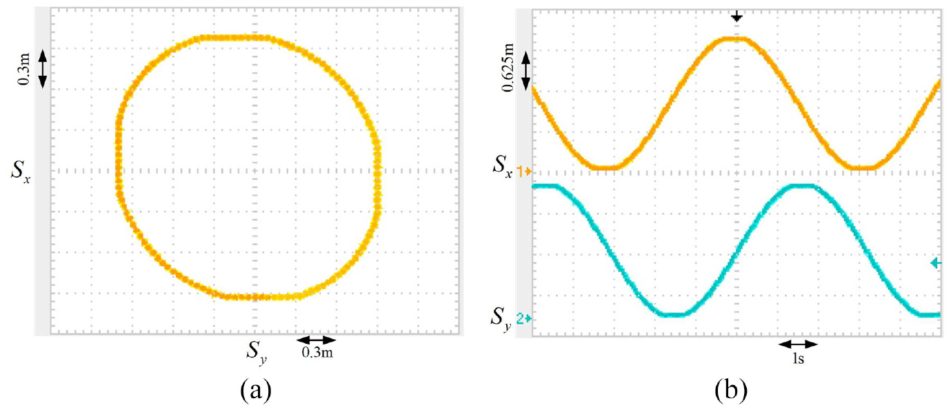
(a) Circular motion trajectory of magnetic levitation planar motor and (b) decomposition of circular motion trajectory.

To test the turning performance of the float of magnetic levitation planar motor. The float moves according to the hexagon track as shown in Figure 13, decomposes its motion trajectory to the x-axis and y-axis. The parameters of horizontal and vertical coordinates are the same as those in Figure 12.

Figure 13.

(a) Hexagon motion trajectory of magnetic levitation planar motor and (b) decomposition of hexagon motion trajectory.

The experimental results show that the float can complete a circular motion with a circumference of 6.283 m in about 6 s. From the decomposition output of the motion trajectory of the x-axis and y-axis, the distance of 2 m float movement needs 3 s, the speed is about 0.6 m/s, and the dynamic response-ability is superior. The ability to output the preset trajectory is good. In the experiment of angle turning, the float completes a hexagon trajectory movement in about 6 s, and its turning process is fast, stable, and not overshoot. Finally, the float control experiment of the maglev planar motor proves that the device has ideal response speed, strong robustness, and good dynamic tracking performance. It is applied in the logistics transmission system described in this article and has a good effect.

Summary and prospect

In this article, the magnetic levitation planar motor is applied to the field of logistics transmission. Taking the model of the magnetic levitation planar motor as the object. Some research on its modeling and controller are made.

Taking the magnetic levitation planar motor model as the object, the mathematical model of thrust and torque of MLPM is analyzed. The current distribution strategy of the coil group and the force/current model is obtained.

According to the characteristics of the linear system, the adaptive controller is designed based on contraction theory. The error between the actual value and the estimated value of the uncertain parameter is limited in the region that meets the contraction characteristic.

Compared with the traditional PID control, the incremental stability analysis based on contraction theory makes the control system get rid of the dependence on the balance point. At the same time, it proves its robustness in the case of uncertain model parameters, which provides a new idea for the further application of magnetic levitation planar motor in logistics.

Footnotes

Acknowledgements

The authors are grateful to the participants of the project for their cooperation.

Handling Editor: James Baldwin

Declaration of conflicting interests

The author(s) declared no potential conflicts of interest with respect to the research, authorship, and/or publication of this article.

Funding

The author(s) disclosed receipt of the following financial support for the research, authorship, and/or publication of this article: This research was funded by National Natural Science Foundation of China (51809128) and National Defense Basic Pre-research Program (jcky2017414c002).

ORCID iD

Guanjun Yang

References

Alimohammadi

Alagoz

Tepljakov

, et al. A NARX model reference adaptive control scheme: improved disturbance rejection fractional-order PID control of an experimental magnetic levitation system. Algorithms 2020; 13: 201.

Bonnabel

Slotine

J-J

. A contraction theory-based analysis of the stability of the deterministic extended Kalman filter. IEEE Trans Automat Control 2015; 60: 565–569.

Chiang

M-L

L-C

. Adaptive stabilization of a class of uncertain switched nonlinear systems with backstepping control. Automatica 2014; 50: 2128–2135.

Han-Sam

Chang-Hwan

Hyun-Kyo

. Magnetic field analysis of 2-D permanent magnet array for planar motor. IEEE Trans Magnet 2001; 37: 3762–3766.

Wang

Zhu

, et al. Performance-oriented precision LARC tracking motion control of a magnetically levitated planar motor with comparative experiments. IEEE Trans Ind Electron 2016; 63: 5763–5773.

Huang

Zhou

Kim

. Minimization design of normal force in synchronous permanent magnet planar motor with Halbach array. IEEE Trans Magnet 2008; 44: 1526–1529.

Huang

Yang

, et al. Integrated robust tracking controller design for a developed precision planar motor with equivalent disturbances. IET Control Theory Appl 2016; 10: 1009–1017.

Kou

Xing

Zhang

, et al. Improved ADRC for a maglev planar motor with a concentric winding structure. Appl Sci 2016; 6: 419.

Sun

Jin

Chen

, et al. Disturbance rejection based on iterative learning control with extended state observer for a four-degree-of-freedom hybrid magnetic bearing system. Mech Syst Signal Process 2021; 153: 107465.

10.

Sun

Jin

Cai

, et al. Grey wolf optimization algorithm based state feedback control for a bearingless permanent magnet synchronous machine. IEEE Trans Power Electron 2020; 35: 13631–13640.

11.

Lahdo

Strohla

Kovalev

. Design and implementation of an new 6-DoF magnetic levitation positioning system. IEEE Trans Magnet 2019; 55: 1–7.

12.

Wang

Tang

, et al. High precision six-degree-of-freedom planar motor control method based on sliding mode control theory. In: International conference on electrical machines and systems, Harbin, China, 11–14 August 2019, pp.1–5. Piscataway, NJ: IEEE.

13.

Lin

Chen

. SoPC-based adaptive PID control system design for magnetic levitation system. IEEE Syst J 2011; 5: 278–287.

14.

Lin

F-J

Teng

L-T

Shieh

P-H

. Intelligent adaptive backstepping control system for magnetic levitation apparatus. IEEE Trans Magnet 2007; 43: 2009–2018.

15.

Wang

Tan

, et al. Adaptive integral backstepping controller for PMSM with AWPSO parameters optimization. Energies 2019; 12: 2596.

16.

Liu

Tian

Wang

, et al. Finite-time control for high-precision tracking in robotic manipulators using backstepping control. IEEE Trans Ind Electron 2016; 63: 5501–5513.

17.

Sun

Shi

Chen

, et al. Internal model control for a bearingless permanent magnet synchronous motor based on inverse system method. IEEE Trans Energy Convers 2016; 31: 1539–1548.

18.

Nguyen

Kim

W-J

. Two-phase Lorentz coils and linear Halbach array for multiaxis precision-positioning stages with magnetic levitation. IEEE/ASME Trans Mechatron 2017; 22: 2662–2672.

19.

Pranayanuntana

Vanchai

. Nonlinear backstepping control design applied to magnetic ball control. In: IEEE region 10 conference, Kuala Lumpur, Malaysia, 2000, pp.304–307. Piscataway, NJ: IEEE.

20.

Shao

Meng

Chen

, et al. The exponential reaching law sliding mode control of magnetic levitation system. In: 2016 Chinese control and decision conference (CCDC), Yinchuan, China, 28–30 May 2016, pp.3500–3503. Piscataway, NJ: IEEE.

21.

Sharma

Kar

. Observer-based synchronization scheme for a class of chaotic systems using contraction theory. Nonlinear Dynam 2010; 63: 429–445.

22.

SungJun

Seo

. Design and analysis of the nonlinear feedback linearizing control for an electromagnetic suspension system. IEEE Trans Control Syst Technol 1997; 5: 135–144.

23.

Thanh

HLNN

Mung

, et al. Perturbation observer-based robust control using a multiple sliding surfaces for nonlinear systems with influences of matched and unmatched uncertainties. Mathematics 2020; 8: 1371.

24.

Tian

Yang

. Adaptive stabilization of a fractional-order system with unknown disturbance and nonlinear input via a backstepping control technique. Symmetry 2019; 12: 55.

25.

Sun

Chen

Jiang

, et al. High-performance control for a bearingless permanent-magnet synchronous motor using neural network inverse scheme plus internal model controllers. IEEE Trans Ind Electron 2016; 63: 3479–3488.

26.

Xing

Kou

Zhang

, et al. Levitation force control of Maglev permanent synchronous planar motor based on multivariable feedback linearization method. In: International conference on electrical machines and systems, Hangzhou, China, 22–25 October 2014, pp.1318–1321. Piscataway, NJ: IEEE.

27.

Yang

, et al. Event-triggered containment control of multi-agent systems with high-order dynamics and input delay. Electronics 2018; 7: 343.

28.

Zhang

Kou

Jin

, et al. Modeling and analysis of a new cylindrical magnetic levitation gravity compensator with low stiffness for the 6-DOF fine stage. IEEE Trans Ind Electron 2015; 62: 3629–3639.

29.

Jiang

Wang

. Incipient winding fault detection and diagnosis for squirrel-cage induction motors equipped on CRH trains. ISA Trans 2020; 99: 488–495.

30.

Zhu

Shi

Abdelwahed

. End-to-end system level modeling and simulation for medium-voltage DC electric ship power systems. Int J Naval Arch Ocean Eng 2018; 10: 37–47.

Magnetic levitation planar motor and its adaptive contraction backstepping control for logistics system

Abstract

Keywords

Introduction

Structure and system modeling of magnetic levitation planar motor

Principle of magnetic levitation planar motor

Mathematical model of magnetic levitation planar motor

Application of magnetic levitation planar motor in logistics transmission

Force/current model of magnetic levitation planar motor

Adaptive contraction backstepping control of magnetic levitation planar motor

Dynamic model of magnetic levitation planar motor

Design of adaptive contraction backstepping controller for MLPM

Basic principle of contraction theory

Design of contraction backstepping controller

Design of adaptive contraction backstepping controller

Experimental verification

Summary and prospect

Footnotes

Acknowledgements

Declaration of conflicting interests

Funding

ORCID iD

References