Sage Journals: Discover world-class research

Abstract

With economic growth, automobiles have become an irreplaceable means of transportation and travel. Tires are important parts of automobiles, and their wear causes a large number of traffic accidents. Therefore, predicting tire life has become one of the key factors determining vehicle safety. This paper presents a tire life prediction method based on image processing and machine learning. We first build an original image database as the initial sample. Since there are usually only a few sample image libraries in engineering practice, we propose a new image feature extraction and expression method that shows excellent performance for a small sample database. We extract the texture features of the tire image by using the gray-gradient co-occurrence matrix (GGCM) and the Gauss-Markov random field (GMRF), and classify the extracted features by using the K-nearest neighbor (KNN) classifier. We then conduct experiments and predict the wear life of automobile tires. The experimental results are estimated by using the mean average precision (MAP) and confusion matrix as evaluation criteria. Finally, we verify the effectiveness and accuracy of the proposed method for predicting tire life. The obtained results are expected to be used for real-time prediction of tire life, thereby reducing tire-related traffic accidents.

Keywords

Automobile tire wear tire life prediction image processing machine learning mean average precision

Introduction

With the development of the automotive industry, vehicles have gradually become the main means of transportation for most people. Therefore, safe driving of vehicles has also become a focus issue. At present, more than half of traffic accidents on highways are caused by tire wear problems, many of which are caused by punctured tires. The main causes of tire perforation are severe surface wear and abnormal tire pressure, which is most likely to occur in the case of high-speed driving or sudden braking. As a main component of cars, tires have a great impact on the performance of vehicles when they are running.¹ Therefore, the detection of tires can effectively improve the safety of vehicles.

In the past few years, manual inspection has been the main technique used to detect the degree of tire wear. A mainstream method is to define the degree of tread pattern wear by detecting the tread depth and the pattern wear of the shoulder, which combines a mathematical model of the tire and local friction and determines the tire wear rule through experiments.^2–5 Another common method is to implant a radio frequency identification (RFID) chip into the tire. Signals from the RFID chip are read by the RFID reader to predict tire wear.^6,7 In addition, the tire model established by finite element method is also often used to simulate abnormal tire wear.^8–10

However, these methods are too expensive to use in a family car. Additionally, technicians need to manually inspect each tire of the vehicle, so the efficiency is not high. In this paper, we use image processing and machine learning techniques to solve this problem. We train the prediction model and use it in tire life experiments, and then select the appropriate evaluation criteria to judge the accuracy of the prediction model. The flow chart of the method is shown in Figure 1.

Figure 1.

Flow chart of the method.

We build a mathematical model of tire wear and mileage, and train the model to predict the life of tire samples. The main steps are as follows.

We build an image library of automobile tire pattern wear and screen tire tread patterns from three brands commonly found in the market. According to the mileage actually used, we divide tires into five categories.

We use appropriate image preprocessing methods to process the completed samples, including normalization, grayscale, median filtering, and histogram equalization, to generate an input sample of the prediction model.

We apply the GGCM and GMRF¹¹ to extract the wear texture features of the input samples.

We employ the KNN¹² classifier cross-validation method to determine the K value and distance formula of the classifier. Then, we build a mapping model of feature vectors and input sample output categories as the life prediction model of this method.

We utilize test samples to verify the performance of the life prediction model. Herein, we use the MAP and confusion matrix as the evaluation methods for the evaluation results.

The remainder of this paper is organized as follows: in Sect. 2, we introduce the theoretical method of the predictive model of this paper. In Sect. 3, we introduce the main influencing factors of the model and conduct experimental verification of the model. In Sect. 4, we give the experimental results and select appropriate evaluation indicators to evaluate the experimental results. Finally, we conclude the paper in Sect. 5.

Theoretical approach

In this section, we introduce the theory of building predictive models. According to the collected image database of car tire pattern wear, we use image pattern extraction technology to quantify tire patterns with different wear levels to obtain corresponding wear feature vectors. Then, we apply machine learning techniques to build a mathematical model relating the wear feature vectors and the degree of wear.

Image library of automobile tire pattern wear

Referring to the relevant literature, we find that the situation of tire tread wear can be divided into four categories: no wear, light wear, moderate wear, and heavy wear, as shown in Figure 2. In addition, we try to make sure that the same light source and angle are used in the same settings when we take the tire image. After filtering the collected images, the images that do not meet the requirements are deleted, and finally the experimental image library is obtained.

Figure 2.

Tire wear classification chart.

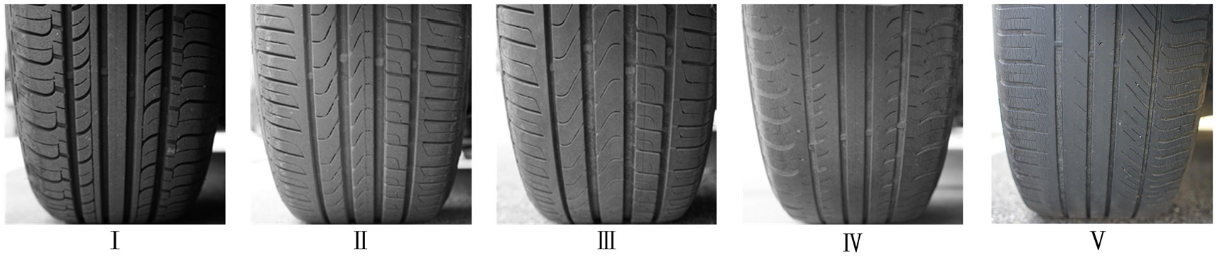
Due to the wide variety of tire brands and patterns in the market, data collection is affected by diverse natural environments and human factors, resulting in an imbalance of data samples. When collecting images, we exclude tires that are damaged due to abnormal use. Meanwhile, we also consider the influence of tire pressure on the data acquisition. We select cars whose tire pressure within the normal using range (2.5 ± 0.3 bar) for sampling. The four tire pressure errors of cars are also within the allowable range (less than 0.1 bar). According to the survey, most of the samples with mileage less than 30,000 km correspond to new cars, while those with more than 60,000 km have been replaced. The new and old tire samples cause large differences in the samples and have a certain impact. Therefore, after multiple screenings, we use the tire tread patterns of three brands common in the market as research objects and divide them into five categories in equal proportions, as show in Figure 3.

Figure 3.

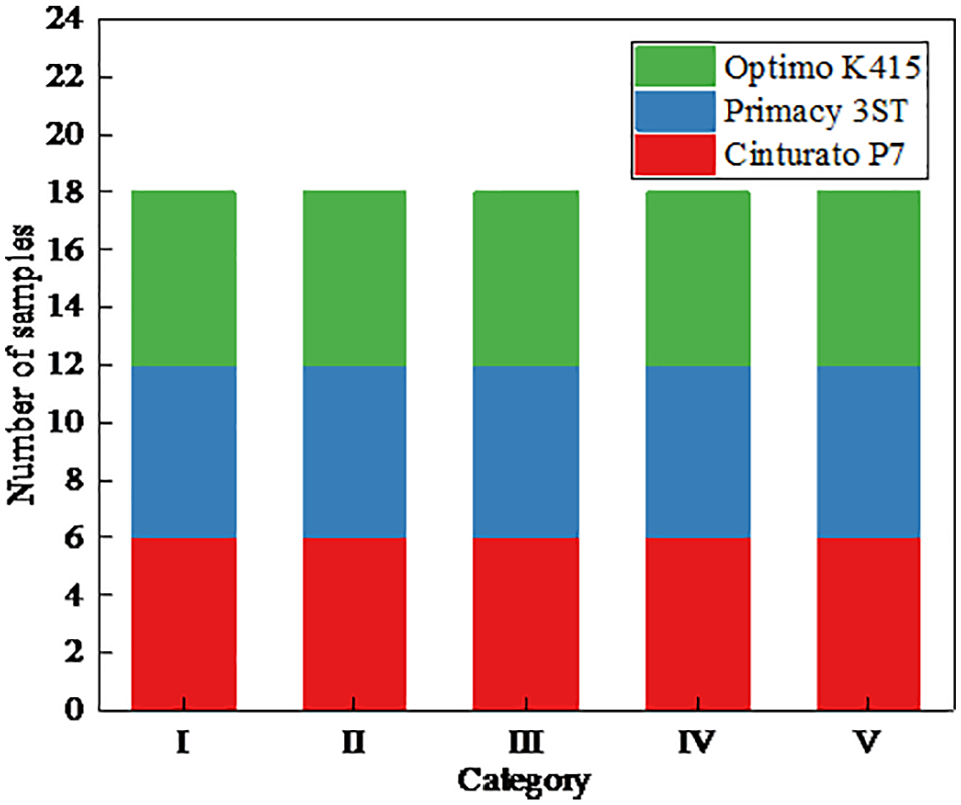
Sample classification map.

We measure tire wear based on their mileage and use that as a classification criterion. The range of the first category of tire is 30,000 to 35,000 km, the second category is 35,000 to 40,000 km, the third category is 40,000 to 45,000 km, the fourth category is 45,000 to 50,000 km, and the fifth type is 50,000 to 60,000 km. The results are shown in Figure 4.

Figure 4.

Classification of tire wear.

To determine whether it makes sense to analyze the three different types of tires, we perform a cluster analysis. As the texture features are high-dimensional, we reduce the dimensions and visualize them. Herein, we use t-distributed stochastic neighbor embedding (t-SNE)¹³ to reduce the dimensions and visualize the data, as shown in Figure 5.

Figure 5.

Tire cluster diagram.

Figure 5 shows that there is an association for the same type of tires (points with the same color in the figure) and that different types of tires (points with different colors in the figure) are different from each other. We can also demonstrate that it makes sense to conduct research on various tire types together.

Image preprocessing

Since the collected original pattern library does not meet the experimental requirements, it is necessary to choose a suitable preprocessing method. We collect the sample images and build a sample library for the experiments. Then, scale normalization and grayscale preprocessing are performed on the collected original images, as shown in Figure 6.

Scale normalization: the original sample size is normalized, and the size is unified to 256 × 256 pixels to ensure the balance of the sample.

Grayscale: the original image is in RGB three-channel mode, and replacing it with a grayscale image can reduce the calculation speed and complexity of feature extraction.

Median filtering:¹⁴ this preprocessing is used to reduce noise caused by the natural environment and human factors during shooting.

Histogram equalization:¹⁵ this preprocessing is used to enhance the contrast of the image, make the gray values of the image evenly distributed, and reduce the influence of uneven illumination during shooting.

Figure 6.

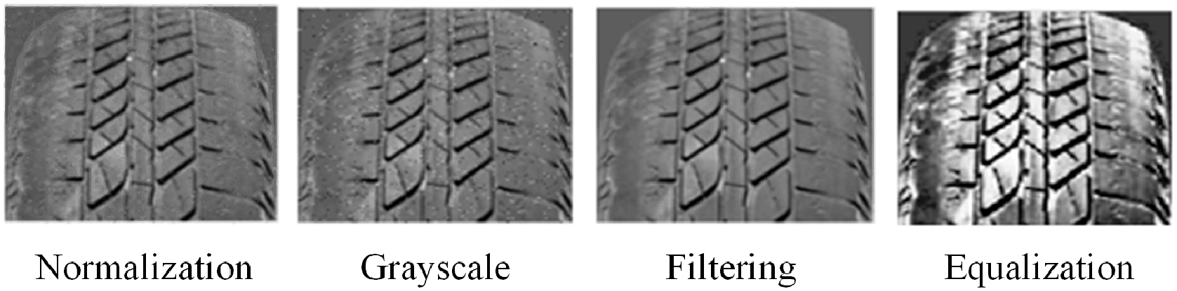
Pretreatment method.

Wear texture feature extraction model

In this subsection, we select and improve algorithms such as GGCM and GMRF to extract texture features from sample images.

Gray gradient co-occurrence matrix

As a classic algorithm for extracting texture features, GGCM is a vital part of the fusion feature extraction model.^16,17 Herein, we briefly introduce the GGCM algorithm. Consider an image with a two-dimensional function of the form:

{f (x, y); x = 1, 2, 3 . . . . N - 1; y = 1, 2, 3 . . . . N - 1},

(1)

where the gradient image is

{g (x, y); x = 1, 2, 3 . . . . N - 1; y = 1, 2, 3 . . . . N - 1} .

(2)

The gradient image is obtained by a gradient operator. If a large number of gray levels lead to a large amount of calculation, then the gray level and the gradient need to be normalized. Then, the normalization to the gray levels of the original image is defined as:

F (x, y) = [f (x, y) (L_{g} - 1) / f_{max}] + 1,

(3)

where [x] is the integer part of x, f_max is the maximum gray level of the original image and L_g is called the grayscale after normalization. The normalization to the gradient image is defined as:

G (x, y) = [g (x, y) (L_{s} - 1) / g_{max}] + 1,

(4)

in which g_max is the maximum gradient of the gradient image and L_s is the gradient scale after normalization. Then, we obtain two matrices after the normalization of the gray levels and gradients as follows:

{G (x, y); x = 1, 2, 3 . . . . N - 1; y = 1, 2, 3 . . . . N - 1},

(5)

{C (i, j); i = 1, 2, 3 . . . L_{g} - 1; j = i = 1, 2, 3 . . . L_{s} - 1},

(6)

where C(i, j) is the number of pixels after normalization, i is the gray level and j is the gradient. The gray-gradient co-occurrence matrix is normalized as:

\hat{C} (i, j) = \frac{C (i, j)}{\sum_{i = 0}^{L_{g} - 1} \sum_{j = 0}^{L_{s} - 1} C (i, j)},

(7)

in which $\sum_{i = 0}^{L_{g} - 1} \sum_{j = 0}^{L_{s} - 1} C (i, j) = N \times N = N^{2}$ .¹⁸

Based on the normalized GGCM, 15 quadratic statistical features can be obtained,^19,20 and their calculation formulas are shown in Appendix A. The GGCM describes the gray and gradient information of pixel points in space.²¹ We use a feature vector composed of the feature parameters T = [T₁, T₂, T₃, T₄, T₅, T₆, T₇, T₈, T₉, T₁₀, T₁₁, T₁₂, T₁₃, T₁₄, T₁₅]^T of the gray-gradient co-occurrence matrix to describe the tire pattern texture with different wear level image features.

Gauss-Markov random field

A Gauss-Markov random field is essentially a set of multidimensional normal score plots and satisfies Markovian random variables.²² Using $x = (x_{1}, x_{2}, . . . . x_{n})^{T}$ to represent a GMRF, we have:

π (x) = (2 π)^{- \frac{n}{2}} {| Q |}^{\frac{1}{2}} \exp (- \frac{1}{2} (x - μ)^{T} Q (x - μ)),

(8)

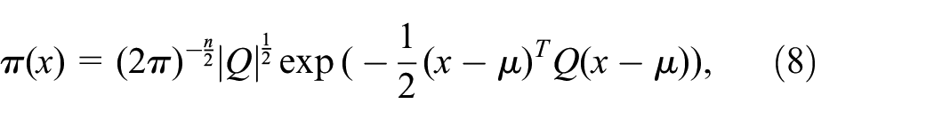
in which Q is the exact matrix and is the inverse of the covariance matrix. The elements at each position determine the nature of x. An element ${Q_{ii}, i = 1, 2, . . ., s}$ on the diagonal determines the conditional accuracy of ${x_{i}, i = 1, 2, . . . ., s}$ and further determines its conditional variance. The off-diagonal elements ${Q_{ij}, i = 1, 2, . . . s, j = 1, 2, . . ., s, i \neq j}$ determine the dependence among the components of x. When $x_{ij} = {x_{1}, . . ., x_{i - 1}, x_{i + 1}, . . ., x_{j - 1}, x_{j + 1}, . . ., x_{n}}$ is given, the correlation coefficient between x_i and x_j is determined, x_i and x_j are independent only when Q_ij =0.

Considering the complexity of tread pattern, parameter performance description and data calculation amount, we adapt the fifth-order GMRF model to describe the texture characteristics of tread pattern under different wear levels. The method is as follows:

Z_{s} = [y_{(i, j) + r_{1}} + y_{(i, j) - r_{1}}, . . ., y_{(i, j) + r_{12}} + y_{(i, j) - r_{1}}],

(9)

where r is the radius of the neighborhood η and {r₁, r₂, r₃, r₄, r₅, r₆, r₇, r₈, r₉, r₁, r₁₀, r₁₁, r₁₂} = {(0, 1), (1, 0), (1, 1), (1, −1), (0, 2), (2, 0), (1, 2), (−1, 2), (2, 1), (−2, 1), (−2, 2), (2, 2)}. Then, we can use a feature vector g = [g₁, g₂, g₃, g₄, g₅, g₆, g₇, g₈, g₉, g₁₀, g₁₁, g₁₂]^T to represent the texture characteristics of tires with different degrees of wear.

K-nearest neighbors and distance formula

The KNN concept utilizes information from measured neighboring points to estimate the unmeasured point values.^23,24 Each uncertain parameter is normalized to eliminate the effect of different value ranges to construct a KNN proxy model.²⁵ Then, the mean value of K closest points is calculated, and a larger weight is given to the closest points to estimate the value of unmeasured points, as shown in equation (10):

z^{\land} ({\vec{θ}}_{0}) = \sum_{i = 1}^{k} λ_{i 0} z ({\vec{θ}}_{i}),

(10)

where ${\vec{θ}}_{0}$ is a vector of independent variables, $z ({\vec{θ}}_{i})$ is the estimated response, ${\vec{θ}}_{i}$ is a vector of the nearest K measured points, $z ({\vec{θ}}_{i})$ is the response of measured points, and $λ_{i 0}$ is the weight function between ${\vec{θ}}_{0}$ and ${\vec{θ}}_{i}$ .²⁶

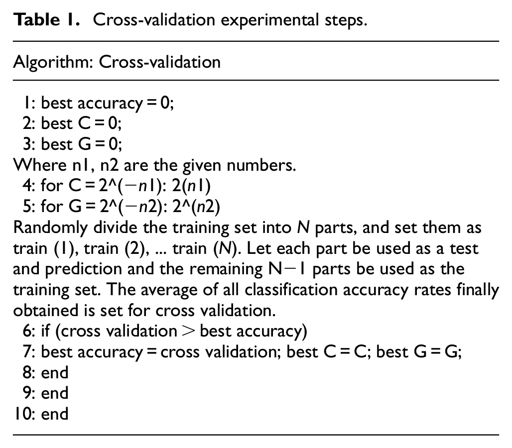
The principle of KNN classification algorithm is to take the samples of all known categories as training groups, calculate the distance between the predicted samples and all known samples, and select the K known samples closest to the unknown samples. According to the majority voting rule, the training sample and KNN were divided into more categories to predict the category of the unknown sample. By calculating the cross-validation loss,^24,27 we choose the best distance formula and K value. First, the samples were randomly divided into several groups, one of which was used as a training sample and the other as a verification sample. Then the training sample is used to train the model, and the verification sample is used to verify the model. Finally, we take the classification accuracy as the performance index of the classifier. The steps are shown in Table 1.

Table 1.

Cross-validation experimental steps.

Algorithm: Cross-validation
1: best accuracy = 0; 2: best C = 0; 3: best G = 0; Where n1, n2 are the given numbers. 4: for C = 2^(−n1): 2(n1) 5: for G = 2^(−n2): 2^(n2) Randomly divide the training set into N parts, and set them as train (1), train (2), … train (N). Let each part be used as a test and prediction and the remaining N−1 parts be used as the training set. The average of all classification accuracy rates finally obtained is set for cross validation. 6: if (cross validation > best accuracy) 7: best accuracy = cross validation; best C = C; best G = G; 8: end 9: end 10: end

Algorithm: Cross-validation

1: best accuracy = 0;
2: best C = 0;
3: best G = 0;
Where n1, n2 are the given numbers.
4: for C = 2^(−n1): 2(n1)
5: for G = 2^(−n2): 2^(n2)
Randomly divide the training set into N parts, and set them as train (1), train (2), … train (N). Let each part be used as a test and prediction and the remaining N−1 parts be used as the training set. The average of all classification accuracy rates finally obtained is set for cross validation.
6: if (cross validation > best accuracy)
7: best accuracy = cross validation; best C = C; best G = G;
8: end
9: end
10: end

This section lists four commonly used distance formulas and chooses the most suitable one. For pixels p, q, and z with coordinates $(x, y)$ , $(s, t)$ , and $(v, w)$ , respectively, if:

(a) $D (p, q) \geq 0 [D (p, q) = 0, p = q]$ ,

(b) $D (p, q) = D (q, p)$ , and

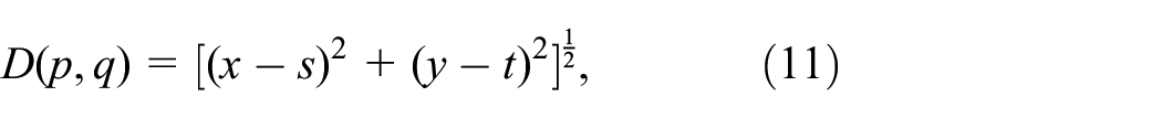
then, D is a distance function or metric. The standardized Euclidean distance²⁸ between p and q is defined as follows:

D (p, q) = [(x - s)^{2} + (y - t)^{2}]^{\frac{1}{2}},

(11)

the city block distance²⁹ between p and q is

D (p, q) = | x - s | + | y - t |,

(12)

the Chebyshev distance³⁰ between p and q is

D (p, q) = max (| x - s |, | y - t |),

(13)

and the Minkowski distance³⁰ between p and q is

D (p, q) = \sqrt[n]{{(x - y)}^{n} + {(s - t)}^{n}} .

(14)

Under cross-validation, we compare the above four different distance formulas and analyze the verification accuracy and cross-loss entropy corresponding to different K values. The results are shown in Figure 7.

Figure 7.

Cross-validation determination distance formula graph.

From Figure 7, with the increase of K value, the loss of cross-validation continues to increase. For experiments in this section, we determine that when K = 1, cross-validation with the Minkowski distance formula has the minimum loss. However, when K = 13, the cross-validation loss increases again, while the cross-validation loss of the city block distance formula is relatively stable. Therefore, we choose the city block distance formula and K = 1 as the KNN classifier parameter in subsequent experiments.

Experiment

This section briefly describes the important parameters of tire features in the feature extraction model and the weight distribution of the fused features. After establishing a theoretical analysis of the life prediction model, we conduct experiments to verify the accuracy of the model. Before the experiments, we separate the training samples from the test samples. We then repeat the experiments with different proportions of training and test samples to obtain the average accuracy.

Parameters of tire features

The gradient is defined as a vector, which means that the directional derivative of the function at that point is maximized in that direction. As can be seen from Figure 8, with the increase of mileage, the tire surface texture gradient presents an upward trend, which means that as the mileage increases, the texture characteristics of the tires will change significantly, and the wear on the tire surface will not be equal. This has certain influence on the study of tire surface texture characteristics.

Figure 8.

Gradient graph.

The difference moment reflects the sharpness of the image and the depth of the texture grooves. The deeper the texture grooves, the greater the contrast and the clearer the visual effect. The larger the gray difference, the larger the value of the difference moment. The inverse difference moment reflects the homogeneity of image texture and measures the variation of image texture locally. A large value indicates that there is no variation between different areas of the image texture, reflecting that this part is very uniform. Figure 9 shows that as the mileage increases, the values of the difference moment and inverse difference moment gradually decrease, indicating that the texture features of tire surface become increasingly fuzzy.

Figure 9.

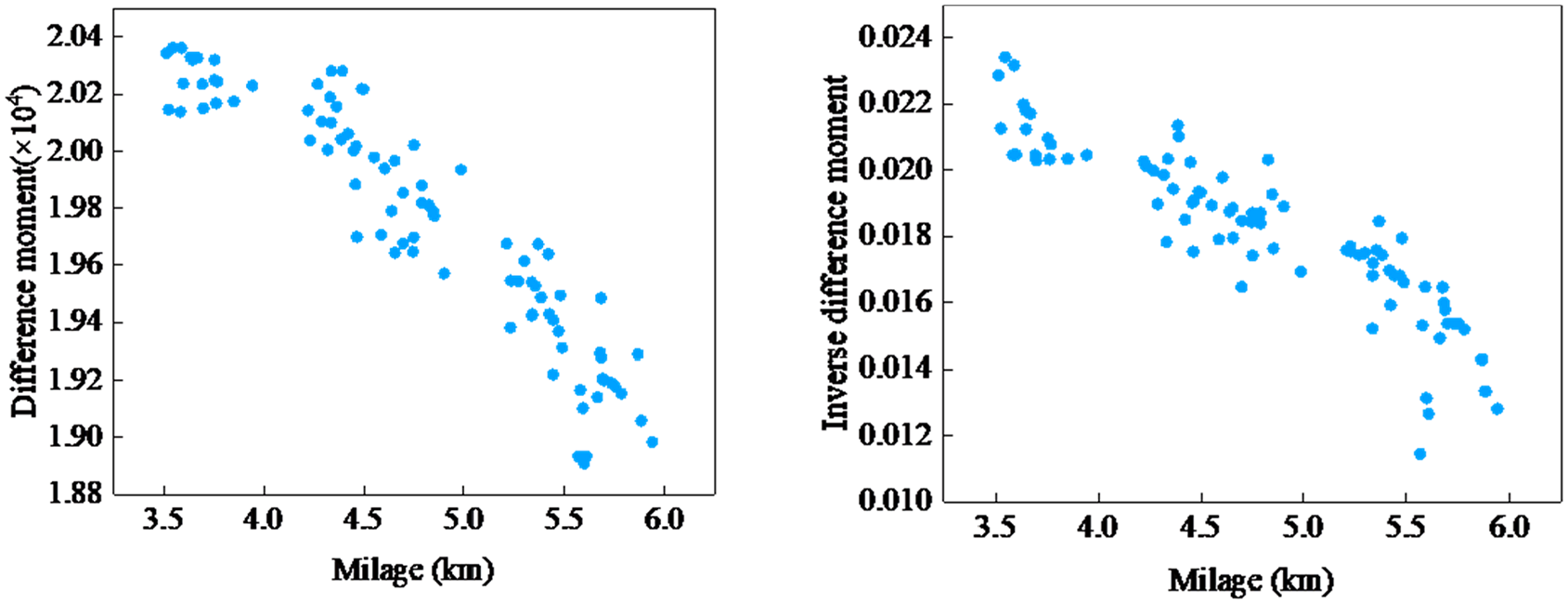
Difference moment and inverse difference moment graph.

According to the characteristics of entropy: the greater the entropy corresponding to a single random variable, the greater the amount of information contained. The entropy value of an image changes with the richness of the gray-scale information of the pixels it contains, the greater the amount of information in the image, the greater it is. The mixed entropy is a second-order statistic derived from GGCM, which can be used as a feature to describe different degrees of tire texture wear. As shown in Figure 10, the three tires are Optimo K415, Cinturato P7, and Primacy 3ST respectively. It is clear that the Optimo K415 texture is much more complex than the other two textures, which is also reflected by the green point value in Figure 11. The texture of the other two tires is similar, with similar values represented by the blue and red dots in Figure 11.

Figure 10.

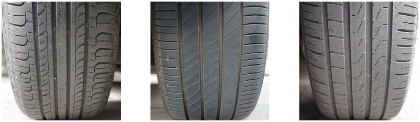
Different model tire maps.

Figure 11.

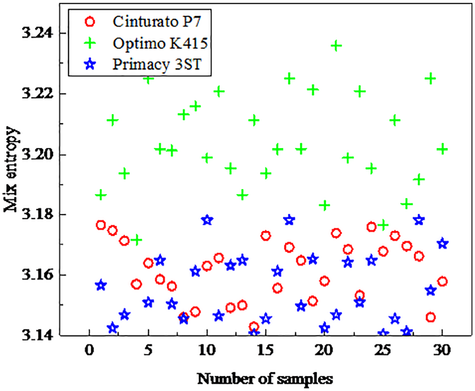
Mixed entropy graph.

According to the entropy theory, the higher the entropy value of the image, the more uniform the gray distribution is. As the entropy of the image increases, the information content of the image increases and the image becomes more complex. The mixed entropy is a second-order statistic derived from GGCM, which can be used to describe the characteristics of tire tread texture with different wear degrees.

Weight allocation of feature extraction model fusion features

In this subsection, we combine the two features of the GGCM and GMRF and assign multiple feature weights to the experiments. Then, we obtain a fusion feature that describes the degree of wear at different angles of the tread pattern, as shown in Figure 12. As can be seen from the results, when x = 0.7 and y = 0.3, the accuracy is the highest, but the fluctuation range is large. When x = 0.4 and y = 0.6, the accuracy decreases slightly, but the fluctuation range is small and the result is stable. In addition, we also provide a comparison diagram of the classification results of single features and fusion features, as shown in Figure 13. This section verifies whether a single feature or a fusion feature should be selected for classification. Compared with the results of single feature classification, the accuracy of fused feature classification is improved to more than 90%.

Figure 12.

Weight distribution experiment chart.

Figure 13.

Comparison of single and fused feature classification results.

The weight ratio of each feature component of the GGCM and GMRF is selected as 4:6. To avoid the influence of different value ranges and dimensions of the two features, the standard normalization method is adopted, as shown in equation (15):

x_{new} = \frac{x - μ}{σ},

(15)

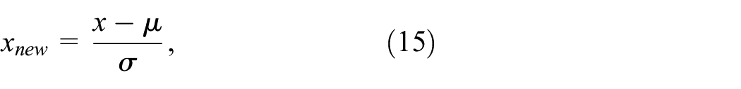
where $μ$ is the mean of the sample and $σ$ is the standard deviation of the sample.

After normalization, the values of the sample data are limited to (0, 1), which matches the standard normal distribution. The steps of feature fusion and weight allocation are as follows:

(1) Let F be the fusion feature of the weights to be assigned, as shown in equation (16):

F = [x \times GGCM, y \times GMRF] .

(16)

(2) Set the step size as 0.1, we traverse all x and y values and calculate the average classification rate of the classifier.

(3) Select the four weight combinations with the highest average classification rates, corresponding to 30, 35, 40, and 45 test samples.

(4) According to variance analysis, if a feature does not diverge, that is, the variance is close to 0, then the influence of the feature in the sample is very small and it is meaningless to distinguish the sample. Therefore, from the four groups of weight combinations, we choose the group with the largest mean variance as the weight coefficient of fusion features.

Results

In this section, we choose the MAP and confusion matrix as the evaluation indicators of the experimental results.

Sample classification and experimental testing

According to the different proportions of the test group and the training group (0.5, 0.6, 0.8, and 1.0), we divided the collected sample database. Different training groups were used to train the model, and different test groups were used to test the model, so as to obtain the average accuracy and running time of the model. The experimental results are shown in Figure 14. The abscissa represents the number of the test image, and the ordinate represents the classification of wear degree. In the same abscissa, the red asterisk shows the predicted classification result, the blue circle indicates the true classification result, the overlap of two points indicates that the predicted classification result is correct, and the absence of overlap indicates that the predicted classification is incorrect. For example, in the resulting image in the upper right corner of Figure 14, the true classification of the first test image is the fourth category represented by a blue circle, and the predicted classification is the fourth category represented by a red asterisk. These two points overlap, indicating that the prediction of the first test image is correct. Table 2 lists the precision and time spent on different scale models. The prediction time of the model is short (average 5–6 s) and the average precision is high (average precision is more than 80%).

Figure 14.

Test model result graph.

Table 2.

Experimental results and operating conditions.

Prediction model number	Test set to training set ratio	Mean average precision %	Time (s)
1	0.5	92.00	5.28
2	0.6	91.42	5.32
3	0.8	87.50	5.44
4	1.0	84.44	5.68
Hardware configuration: i5 CPU, 8 GB memory
Operating environment: MATLAB R2018b
KNN parameter: K = 3; city block distance; Number of training samples: 30

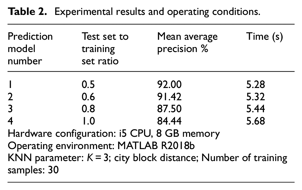
The verification model conditions are shown in Table 2: an i5 CPU, 8 GB running memory, MATLAB R2018b operating environment, KNN classifier (K = 3), city block distance, and 30 verifications per group. It should be noted that the K value of KNN classifier is different from that of theoretical analysis. When K = 3, the prediction model has the highest accuracy.

Evaluation of experimental results

After obtaining the results through experiments, we perform a series of evaluations, such as for the accuracy of the results. This section introduces two evaluation methods and applies them to the model.

Mean average precision

In measuring the performance of a model, it is unscientific to use precision or recall alone. Next, we introduce MAP as an evaluation indicator.

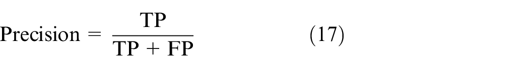
We define categories that are identified and correctly classified as true positive (TP) but incorrectly classified as false positive (FP), categories that are not correctly identified and classified as true negative (TN), and categories that are uncertain but incorrectly classified as false negative (FN). Equation (17) can be used to calculate the accuracy and equation (18) is used to calculate the recall rate.

Precision = \frac{TP}{TP + FP}

(17)

Re call = \frac{TP}{TP + FN}

(18)

We draw a two-dimensional curve of precision and recall, use them as the vertical and horizontal coordinates, respectively, and name them PR curve. Then, we use the PR curve under area as a measure. Finally, we have the concept of average precision (AP). Its calculation formula is shown in equation (19):

AP = \int_{0}^{1} P (r) dr

(19)

The mean average precision, which is the average of AP values, is the AP values for multiple validation sets.³¹ The MAP calculation formula is shown in equation (20):

MAP = \frac{1}{n} \sum_{1}^{n} AP

(20)

Classification accuracy rate is the ratio of the number of correctly classified samples to the total number of samples in a given sample. However, the accuracy is not applicable to uneven data. For example, in a binary classification problem, we have 1000 samples, of which 10 are positive samples and 990 are negative samples. If all samples are directly classified as negative, then the accuracy is 99%, while the positive samples are all wrong, so the classification performance of the model is actually very poor. For experiments in this section, we choose random test samples and training samples that will lead to data imbalance. The accuracy of evaluation cannot accurately describe the classification performance of the model. Therefore, the confusion matrix is used to further study the classification performance of the model.

Confusion matrix

The confusion matrix is a case analysis table that summarizes the predicted results of the classification models in machine learning. The records in the data set are summarized in the form of matrix according to the two criteria of the real category and category judgment predicted by the classification model. The rows of the confusion matrix represent the true values and the columns represent the predicted values. All the correct predictions are on the diagonal, so it is convenient and intuitive to see what is wrong with the confusion matrix and why the values appear outside the diagonal. As shown in Figure 15, the numerator value of the precision is the value on the diagonal of the matrix.³²

Figure 15.

Confusion matrix diagram.

Evaluation of experimental results

The confusion matrix is calculated by comparing the position of each measured pixel with the corresponding position in the classified image. In Figure 16, the abscissa indicates the expected classification result, and the ordinate indicates the actual classification result. The overlapping of the two indicates that the classification is correct. It can be seen that during classification, only the first and fourth types have allowable errors, and the accuracy of the other classification results is above 80%, indicating that this method can accurately predict tire life.

Figure 16.

Model classification result confusion matrix.

By using the MAP and confusion matrix to verify the experimental results, it can be seen that the model shows good accuracy in tire life prediction.

Conclusion

This paper presents a novel method for predicting the life of automobile tires. Firstly, we establish an original image database and perform preprocessing and texture feature extraction on the original image. Secondly, we input the extracted features into the classifier to train and test the model. Finally, we use appropriate evaluation indicators to analyze the accuracy of the model.

Experiments demonstrate that the proposed method shows high accuracy, fast efficiency and low cost in predicting tire life. However, there are still some shortcomings in this study. For example, factors such as road conditions, tire size, and tire quality require further consideration. Moreover, this article only makes experimental predictions based on small sample data, and this work needs to be extended to large sample tests. We will report on these results in future publications.

Footnotes

Appendix A

In this appendix, we introduce the 15 parameters describing the GGCM extraction of texture feature, they are: small gradient advantage, large gradient advantage, gray distribution unevenness, gradient distribution unevenness, energy, gray average, gradient average, gray mean square error, gradient mean square error, correlation, gray entropy, gradient entropy, mixed entropy, difference moment, and inverse difference moment. Their calculation formulas are:

(21)

T_{1} = [\sum_{i = 0}^{N_{H}} \sum_{j = 0}^{N_{g}} \frac{g (i, j)}{j^{2}}] / [\sum_{i = 0}^{N_{H}} \sum_{j = 0}^{N_{g}} g (i, j)],

(22)

T_{2} = [\sum_{i = 0}^{N_{H}} \sum_{j = 0}^{N_{g}} j^{2} g (i, j)] / [\sum_{i = 0}^{N_{H}} \sum_{j = 0}^{N_{g}} g (i, j)],

(23)

T_{3} = {\sum_{i = 0}^{N_{H}} {[\sum_{j = 0}^{N_{g}} g (i, j)]}^{2}} / [\sum_{i = 0}^{N_{H}} \sum_{j = 0}^{N_{g}} g (i, j)],

(24)

T_{4} = {\sum_{j = 0}^{N_{g}} {[\sum_{i = 0}^{N_{H}} g (i, j)]}^{2}} / [\sum_{i = 0}^{N_{H}} \sum_{j = 0}^{N_{g}} g (i, j)],

(25)

T_{5} = \sum_{i = 0}^{N_{H}} \sum_{j = 0}^{N_{g}} {[P (i, j)]}^{2},

(26)

T_{6} = \sum_{i = 0}^{N_{H}} i \cdot [\sum_{j = 0}^{N_{g}} P (i, j)],

(27)

T_{7} = \sum_{j = 0}^{N_{g}} j \cdot [\sum_{i = 0}^{N_{H}} P (i, j)],

(28)

T_{8} = \sqrt{\sum_{i = 0}^{N_{H}} {(i - T_{6})}^{2} \cdot \sum_{j = 0}^{N_{g}} P (i, j)},

(29)

T_{9} = \sqrt{\sum_{j = 0}^{N_{g}} (j - T_{7}) \cdot \sum_{i = 0}^{N_{H}} P (i, j)},

(30)

T_{10} = \frac{1}{T_{8} \cdot T_{9}} \sum_{i = 0}^{N_{H}} \sum_{j = 0}^{N_{g}} (i - T_{6}) (j - T_{7}) P (i, j),

(31)

T_{11} = - {\sum_{i = 0}^{N_{H}} [\sum_{j = 0}^{N_{g}} P (i, j)] \cdot \log [\sum_{j = 0}^{N_{g}} p (i, j)]},

(32)

T_{12} = - {\sum_{j = 0}^{N_{g}} [\sum_{i = 0}^{N_{H}} P (i, j)] \cdot \log [\sum_{i = 0}^{N_{H}} p (i, j)]},

(33)

T_{13} = - \sum_{i = 0}^{N_{H}} \sum_{j = 0}^{N_{g}} P (i, j) \cdot \log (P (i, j)),

(34)

T_{14} = \sum_{i = 0}^{N_{H}} \sum_{j = 0}^{N_{g}} {(i - j)}^{2} P (i, j),

(35)

T_{15} = \sum_{i = 0}^{N_{H}} \sum_{j = 0}^{N_{g}} \frac{1}{1 + {(i - j)}^{2}} P (i, j),

where i and j are the coordinates of the pixel in the digital image, P(i, j) and g(i, j) are the values of the coordinates.

Handling Editor: James Baldwin

Declaration of conflicting interests

The author(s) declared no potential conflicts of interest with respect to the research, authorship, and/or publication of this article.

Funding

The author(s) disclosed receipt of the following financial support for the research, authorship, and/or publication of this article: The work reported in this paper was supported by the National Natural Science Foundation of China under Grant No. 11602142.

ORCID iD

Shenlong Wang

References

Cui

Liu

Zhang

, et al. Tire defects classification with multi-contrast convolutional neural networks. Int J Pattern Recognit Artif Intell 2018; 32: 1850011.

Chen

Guo

Tire wear estimation based on nonlinear lateral dynamic of multi-axle steering vehicle. Int J Automot Technol 2018; 19: 63–75.

Huang

Chiu

Y-J

Jin

X-x.

Numerical calculation of irregular tire wear caused by tread self-excited vibration and sensitivity analysis. J Mech Sci Technol 2013; 27: 1923–1931.

Lupker

Cheli

Braghin

, et al. Numerical prediction of car tire wear. Tire Sci Technol 2004; 32: 164–186.

Muhamedsalih

Stow

Bevan

Use of railway wheel wear and damage prediction tools to improve maintenance efficiency through the use of economic tyre turning. Proc Inst Mech Eng Part F: J Rail Rapid Transit 2019; 233: 103–117.

Shiao

CS.

Development of an onboard automatic tire-wear warning system. Appl Mech Mater 2013; 284–287: 1821–1825.

Hong

Yang

Implantable electronic tag for tire and assembly process. Patent US 2019/0205722 A1, U.S., 2019.

Wang

, et al. Finite element analysis for tire tread wear under typical loading conditions. In: The third international conference on mechanical engineering and mechanics, Beijing, China, 2009, pp.884–888. http://apps.webofknowledge.com/full_record.do?product=UA&search_mode=GeneralSearch&qid=1&SID=6Dd9R52QT6gQMgmUHsO&page=1&doc=1

Zuo

, et al. Prediction procedure for wear distribution of transient rolling tire. Int J Automot Technol 2014; 15: 505–515.

10.

Nguyen

Zheng

Schmerwitz

, et al. An advanced abrasion model for tire wear. Wear 2018; 396: 75–85.

11.

Almakady

Mahmoodi

Bennett

. Gaussian Markov random fields-based features for volumetric texture segmentation. In: 2019 IEEE conference on multimedia information processing and retrieval (MIPR) 2019, pp.212–215. IEEE. https://ieeexplore.ieee.org/document/8695349

12.

Shi

Gao

Wang

Transductive cost-sensitive lung cancer image classification. Appl Intell 2013; 38: 16–28.

13.

Linderman

Steinerberger

Clustering with t-SNE, provably. SIAM J Math Data Sci 2019; 1: 313–332.

14.

Villar

Torcida

Acosta

GG.

Median filtering: a new insight. J Math Imaging Vision 2017; 58: 130–146.

15.

Mohapatra

Panda

PP.

Histogram equalization and noise removal process for enhancement of image. ACCENTS Trans Image Process Comput Vision 2017; 3: 22-25.

16.

Liu

Dai

, et al. A coverless information hiding algorithm based on grayscale gradient co-occurrence matrix. IETE Tech Rev 2018; 35: 23–33.

17.

Shen

Shi

Chen

Splicing image forgery detection using textural features based on the grey level co-occurrence matrices. IET Image Process 2016; 11: 44–53.

18.

Chen

Jiang

. The research of recognition on oceanic internal waves based on gray gradient co-occurrence matrix and BP neural network. In: 2011 symposium on photonics and optoelectronics (SOPO) Wuhan, China, 31 May 2011, pp.1–4. IEEE. https://ieeexplore.ieee.org/document/5780570

19.

Arya

Singh

Agrawal

RK.

A novel combination of second-order statistical features and segmentation using multi-layer superpixels for salient object detection. Appl Intell 2016; 46: 1–18.

20.

Cui

Wang

Zhang

, et al. A recognition algorithm to detect pipe weld defects. Teh Vjesn 2017; 24: 1969–1975.

21.

Wan

Long

. An inspection method of rice milling degree based on machine vision and gray-gradient co-occurrence matrix. In: International conference on computer and computing technologies in agriculture, Berlin, Heidelberg, 2010, pp.195–202. Springer. https://link.springer.com/chapter/10.1007%2F978-3-642-18333-1_23

22.

Xing

Deng

Xin

, et al. Investigation of a novel automatic micro image-based method for the recognition of animal fibers based on Wavelet and Markov random field. Micron 2019; 119: 88–97.

23.

Ferri

Tomba

Visotti

, et al. A feasibility study for a persistent homology-based k-nearest neighbor search algorithm in melanoma detection. J Math Imaging Vision 2017; 57: 324–339.

24.

Zhang

Zong

, et al. Efficient knn classification with different numbers of nearest neighbors. IEEE Trans Neural Networks Learn Syst 2017; 29: 1774–1785.

25.

Prasath

Alfeilat

HAA

Lasassmeh

, et al. Distance and similarity measures effect on the performance of K-nearest neighbor classifier—a review. arXiv preprint arXiv:170804321 2017: 1–39.

26.

Callahan

Kosaraju

SR.

A decomposition of multidimensional point sets with applications to k-nearest-neighbors and n-body potential fields. J ACM 1995; 42: 67–90.

27.

Koh

JEW

EYK

Bhandary

, et al. Automated detection of retinal health using PHOG and SURF features extracted from fundus images. Appl Intell 2018;48(5): 1379–1393.

28.

Laha

Hazarika

A heuristic approach based on Euclidean distance matrix for the machine-part cell formation problem. Mater Today: Proc 2017; 4: 1442–1451.

29.

Arora

Tushir

Robust spatial intuitionistic fuzzy C-means with city-block distance clustering for image segmentation. J Intell Fuzzy Syst 2018; 35: 5255–5264.

30.

Rodrigues

ÉO

. Combining Minkowski and Cheyshev: new distance proposal and survey of distance metrics using k-nearest neighbours classifier. Pattern Recognit Lett 2018; 110: 66–71.

31.

Qayyum

Anwar

Awais

, et al. Medical image retrieval using deep convolutional neural network. Neurocomputing 2017; 266: 8–20.

32.

Landgrebe

TCW

Duin

RPW

. Efficient multiclass ROC approximation by decomposition via confusion matrix perturbation analysis. IEEE Trans Pattern Anal Mach Intell 2008; 30: 810–822.

Automobile tire life prediction based on image processing and machine learning technology

Abstract

Keywords

Introduction

Theoretical approach

Image library of automobile tire pattern wear

Image preprocessing

Wear texture feature extraction model

Gray gradient co-occurrence matrix

Gauss-Markov random field

K-nearest neighbors and distance formula

Experiment

Parameters of tire features

Weight allocation of feature extraction model fusion features

Results

Sample classification and experimental testing

Evaluation of experimental results

Mean average precision

Confusion matrix

Evaluation of experimental results

Conclusion

Footnotes

Appendix A

Declaration of conflicting interests

Funding

ORCID iD

References