Sage Journals: Discover world-class research

Abstract

This paper analyzed the effects of boundary conditions on the stress distribution of hydraulic support with the static finite element (FE) model. Five loading conditions are considered in this study, including: 1) canopy torsional loading, 2) canopy eccentric loading, 3) base torsional loading, 4) base diagonal loading, and 5) base symmetrical loading. In order to verify the simulation results obtained from the FE model, the corresponding experiments have also been performed. Based on the comparison between simulation and experimental results, the effects of pin-joint simplified methods and boundary conditions are evaluated in terms of accuracy and efficiency. Moreover, the new elastic-support boundary is also proposed to improve the simulation accuracy under conditions 2, 3, 4, and 5. The results show that bonded contact between the pin and shaft hole has high efficiency and accuracy compared with the frictional contact. The frictional contact boundary is reasonable under condition 1. However, the elastic-support boundary is suggested to be adopted to improve calculation accuracy for the stress distribution of the constraint components (canopy or base) under conditions 2, 3, 4, and 5.

Keywords

Hydraulic support boundary conditions strength characteristics finite element experiment

Introduction

The hydraulic support is one of the important safety supporting equipment in the process of coal mining.^1–3 Its safety and reliability are very important for the safe mining of coal mines. In order to improve design quality, many researchers have carried out a lot of research on static strength^4–7 and dynamic behaviors^8–10 of hydraulic support. At present, static strength calculation by equivalent loads is widely used to assure the design quality. Due to the complex structures and loading conditions of hydraulic support, it is difficult to carry out the strength check by material mechanics method. The FE method with the ideas of numerical approximation and discretization has high precision and can deal with large structures with complex shapes,^11–17 such as turbine bladed disks,¹² gear pairs^14,15 and gas formed structures.¹⁶ The FE method has been adopted for calculating the strength of hydraulic support in many researches.^18–29 A FE model needs reasonable simplification and assumptions such as boundary conditions and equivalent treatment of joints to ensure the validity of simulation results. In order to establish the FE model better, the model verification, and modification should be carried out by experiments.¹⁸

Lu et al.¹⁸ established a beam-shell combined the FE model of hydraulic support, in which a pin-joint adopted the beam element, and the other components adopted the shell element. They analyzed the influence of boundary constraints, various loads, and different support heights on the simulated stresses and verified the proposed model with measured stresses. He et al.¹⁹ established an overall FE model of hydraulic support with shell elements and performed the strength simulation analysis under the canopy and base torsional loading conditions respectively. Li et al.²⁰ established a shell-solid combined FE model of hydraulic support, in which the welding among all parts adopted the common use of nodes, and the constraint between the cushion block and canopy or base adopted the frictional contact boundary. Considering the pin-joint with the frictional contact element, Gao and Zhou²¹ also established a similar shell-solid FE model and the constraint boundary is similar to that in Li et al.²⁰ Li²² established a FE model of hydraulic support by using tetrahedral and hexahedral mixed elements, analyzed the stress distribution under the canopy and base concentrated loading conditions respectively, and verified the effectiveness of the simulated results by experiment. Under three loading conditions, Ma et al.^23,24 established a solid FE model of ZF5000/16/28 hydraulic support with a mesh size of 60 mm and compared the simulated stress distribution with that obtained from the experiment. Liu and Liu²⁵ established a 3D FE model of ZT650/19.5/34 hydraulic support and analyzed the stress and deformation distribution of the support under four working conditions.

Based on ABAQUS software, Li and Zheng²⁶ established a FE model of ZF5000/16/28 hydraulic support and analyzed the stress and displacement distribution under the canopy eccentric and base torsional loading conditions by simplifying the pin-joint as coupling hinge, describing the contact between the cushion block and the canopy or the base by contact element, and setting the jack as rigid connection. Based on a bilinear constitutive model, Zhao et al.²⁷ established a static FE model of hydraulic support, and analyzed the static strength of the support and the fatigue characteristics of the welded box structure. Wu et al.²⁸ established a 3D FE model of six-column hydraulic support, and analyzed the stress distribution of each component under the base two-end concentrated and torsional loading conditions, respectively. Kong et al.²⁹ adopted the frictional contact to simulate the rotation of pin-joint, established a FE model of hydraulic support, and analyzed the strength characteristics of the system under three loading conditions.

The above literature survey shows that the boundary conditions for the contact between the canopy/base and working table mainly adopt fixed constraint and frictional contact boundary. Some researchers point out that the frictional contact boundary is consistent with the actual situation. Some simulated results are also verified by experiments. However, it is difficult to accurately assess the influence of boundary conditions on the stress distribution of the whole hydraulic support due to the lack of measured points. In order to bridge this gap, under the canopy torsional loading condition, this paper compares the simulated stress distribution considering different traditional boundary and pin-joint simplification assumptions with measured stress distribution and different pin-joint assumptions. The reason for the error between the simulation and experiment is analyzed. In order to improve the simulation accuracy, a new elastic-support boundary is proposed to simulate the local contact phenomenon caused by eccentric loading, assembly error and unevenness of canopy, on the base and working table surface. This study can provide theoretical support for the accurate evaluation of the stress distribution of hydraulic support.

Finite element model and experiment description of hydraulic support

CAD model simplification and finite element modelling

The actual structure of hydraulic support has many auxiliary parts, such as guard plates and legs. Consequently, before the FE modelling, it is necessary to simplify the CAD model of hydraulic support. The model simplification principles are as follows: ① The non-load bearing parts are removed, such as the canopy protection plate at the left and right sides of the canopy, hydraulic components, etc. Only the key bearing parts such as the canopy, goaf shield, base, front, and rear linkages are retained. ② The load-bearing parts are also removed, such as the lifting ring for mounting hydraulic hoses of the canopy part, the hydraulic cylinders, and the small hydraulic oil ports. ③ Geometrical features of bearing parts are processed, such as deleting the edge chamfering, rounded corners, and processing holes, and filling some welding seams, and fine clearance.

In the experiment, the hydraulic system of hydraulic support provides pressure, and then the positions of the cushion blocks are changed to simulate different loading forms of hydraulic support, so as to evaluate the hydraulic support performance more comprehensively.³⁰

In this paper, only five dangerous conditions are selected to carry out the simulation and experiment: Canopy torsional loading condition is condition 1, and canopy eccentric loading condition is condition 2. The cushion block layouts of condition 1 and condition 2 are shown in Figure 1(a) and (b), and the base is in direct contact with the upper surface of the lower working table. Base torsional loading condition is condition 3, base diagonal loading condition is condition 4, and base symmetrical loading condition is condition 5. The cushion block layouts of conditions 3, 4, and 5 are shown in Figure 1(c) to (e), and the canopy is in direct contact with the upper working table.

Figure 1.

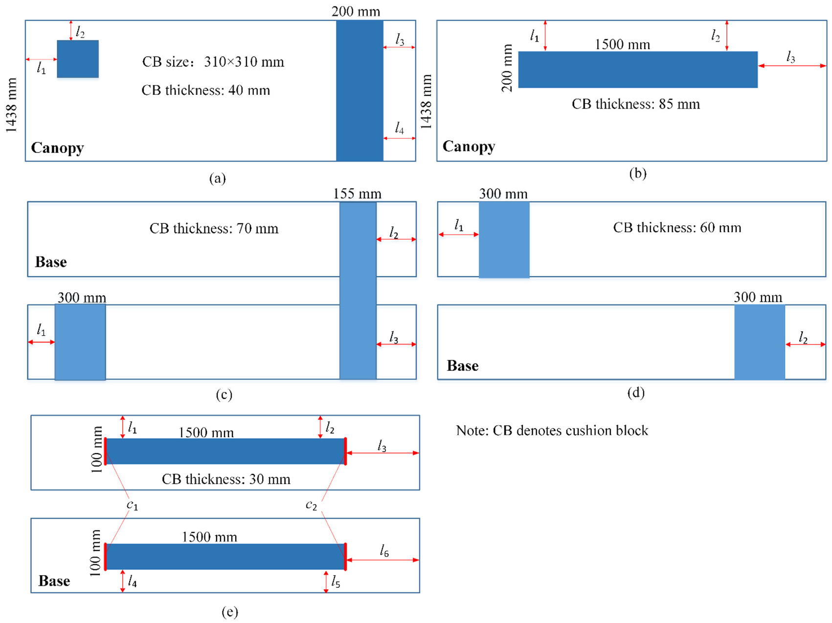
Five loading conditions: (a) condition 1: canopy torsional loading condition, (b) condition 2: canopy eccentric loading condition, (c) condition 3: base torsional loading condition, (d) condition 4: base diagonal loading condition, and (e) condition 5: base symmetrical loading condition.

It should be noted that there are some small differences between the actual conditions and specified conditions in GB 25974.1-2010,³⁰ due to the limitation of the experiment. For example, the small cushion block thickness can lead to the contact between the canopy and working table, so the block thickness is increased by stacking multiple cushion blocks. In addition, the positions of the cushion block may change during the loading process. The detailed parameters during the experiment are provided in Section 2.2.

According to Huangfu,¹⁴ the legs of hydraulic support can be regarded as a two-force bar, which applies a pair of equal and opposite forces to the sockets of the canopy and the base. The rated working pressure of the hydraulic cylinder of the leg is p = 42.3 MPa, and the inner diameter of the cylinder is D = 320 mm. According to the standard of GB25974.1-2010,³⁰ the applied loading of the single leg F is 4080 kN which is set as 1.2 times the rated load. The FE model of hydraulic support is established in ANSYS Workbench. The applied loading and FE model (condition 1) are shown in Figure 2. It should be noted that the equilibrium cylinder has little effect on the static stress of the whole hydraulic support, so the applied force of the equilibrium cylinder is ignored in this paper.³¹ The main structural material of hydraulic support is steel (a Young’s modulus E = 210 GPa, a density ρ = 7850 kg/m³, a Poisson’s ratio υ = 0.3). The FE model of hydraulic support is established by SOLID186 and SOLID187 elements and the element size is set as 35 mm. SOLID186 element is a high order 3-D 20-node solid element, which is used to mesh some regular shaped parts with 6 facets, while SOLID187 is a high order 3-D 10-node solid element, which is used to mesh irregular or complex parts better. Using SOLID186 and SOLID187 elements, not only ensures the FE mesh quality, but also effectively reduces the calculation scale and improves the calculation efficiency.

Figure 2.

(a) Schematic of applied loading and (b) FE model under condition 1.

Different boundary conditions will lead to different finite element simulation results. Therefore, for the above five experiment conditions, how to set the appropriate boundary conditions is the focus of this paper.

Description of experimental equipment and measurement process

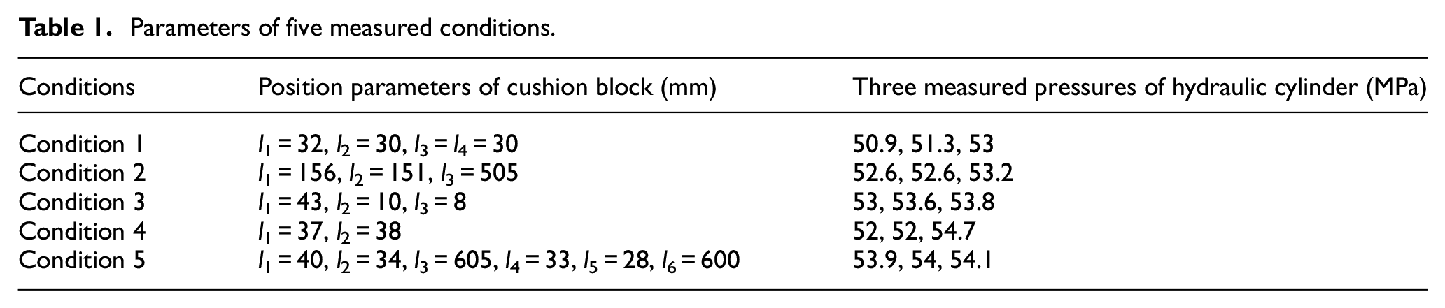
The hydraulic support is tested on a 3000 t hydraulic experiment rig (see Figure 3(a)), and the Von Mises equivalent stresses of the measured points are obtained by the LMS data acquisition instrument (VB8E, DB8 board card, 128 channels) and the strain gauge produced by Zhonghang Electronic Measuring Instruments Co., Ltd (rectangular strain rosette, 120 Ω), as is shown in Figure 3(b). The parameters for five loading conditions are listed in Table 1. Three groups of data are collected, and the average values of Von Mises stresses under the stable state are used as the final experimental results. The photos and position schematic of measured points are shown in Figure 4. It should be noted that auxiliary measured points are added in the region where the stress gradient varies. The measured points are named as follows: three measured points of 23′ (main measured point), 23′′ (auxiliary measured point 1), and 23′′′ (auxiliary measured point 2) are arranged on the canopy. Only one measured point is named as measured point i (i = 1, 10, 12, 13, 25). The number of measured points is discontinuous because some measured points with small stresses are removed, such as measured points 2, 3, 21, and 22.

Figure 3.

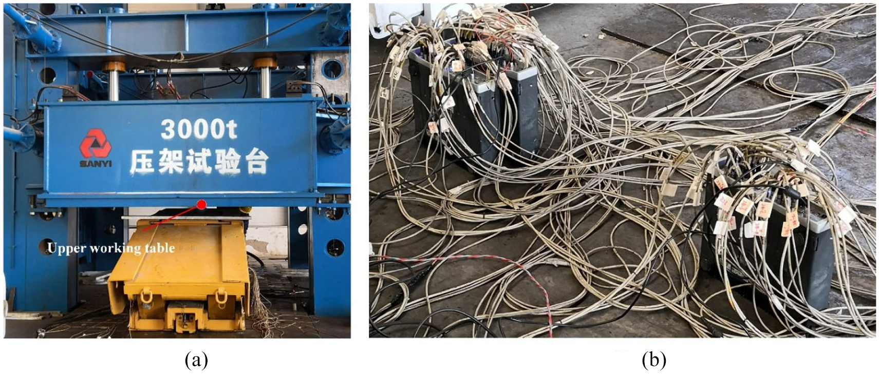
(a) Experiment rig and (b) LMS data acquisition instrument.

Table 1.

Parameters of five measured conditions.

Conditions	Position parameters of cushion block (mm)	Three measured pressures of hydraulic cylinder (MPa)
Condition 1	l ₁ = 32, l₂ = 30, l₃ = l₄ = 30	50.9, 51.3, 53
Condition 2	l ₁ = 156, l₂ = 151, l₃ = 505	52.6, 52.6, 53.2
Condition 3	l ₁ = 43, l₂ = 10, l₃ = 8	53, 53.6, 53.8
Condition 4	l ₁ = 37, l₂ = 38	52, 52, 54.7
Condition 5	l ₁ = 40, l₂ = 34, l₃ = 605, l₄ = 33, l₅ = 28, l₆ = 600	53.9, 54, 54.1

Figure 4.

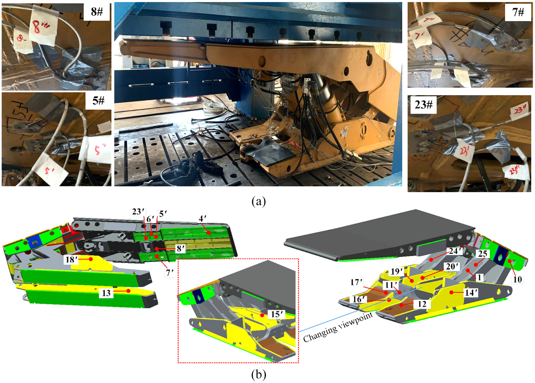
(a) Partial measured points in experiment and (b) schematic of measured point locations.

Taking condition 1 as an example, the Von Mises stress curves of four main and auxiliary measured points are shown in Figure 5. The figure shows that the experiment process has a stable process from the loading, and the stress value tends to be stable after 105 s. The stress in the stable stage is selected as the final experimental result.

Figure 5.

Von Mises stresses of different measured points: (a) 5#, (b) 7#, (c) 8#, and (d) 23#.

The stress gradient of some measured points varies greatly, such as measured point 8# (see Figure 5(c)). There are many welds around this measured point, and both the surrounding structure and the applied load are complex. In order to analyze the deformation of measured point 8# in detail, the uniaxial strain curves in three directions are shown in Figure 6. It can be seen that the variation gradient of uniaxial strains is also large. Compressive strain mainly appears in a-direction, where the strain value is greater than tensile strain, and the compressive strain of measured point 8′ is the largest. The tensile strains of measured point 8′′′ in b-direction and measured point 8′ in c-direction are the largest.

Figure 6.

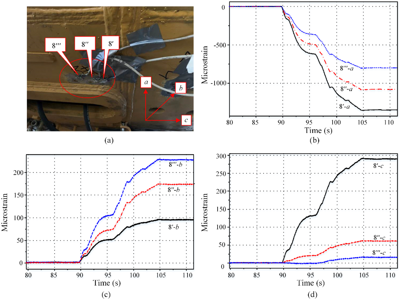
(a) Schematic of three strain directions, (b) microstrain in a-direction, (c) microstrain in b-direction, and (d) microstrain in c-direction.

Comparison of simulated and measured stress under different conditions

Stress comparison under canopy torsional loading condition (condition 1)

The bottom surface of the lower working table is set as fixed constraint during the experiment. For condition 1, the experiment state is indicated by setting the upper surface of cushion blocks as fixed constraint, the bottom surface of cushion blocks as bonded contact, and setting the base as frictional contact with the upper surface of lower working table (in this paper, the friction coefficient is set as 0.2). Li et al.²⁰ shows that such boundary conditions can get results that are more consistent with experimental data. Under the above boundary and loading conditions, four simplified methods of pin-joint will be discussed which are listed in Table 2.

Table 2.

Simplified methods of pin-joint.

Cases	Simplified methods
1.1	Removing pin-joints, the pin-joint connection positions adopt bonded contact
1.2	Removing pin-joints, the pin-joint connection positions adopt revolute joint which can consider local deformation
1.3	Retaining pin-joints, and the pin is bonded with the pinhole
1.4	Retaining pin-joints, the connection between the pin and the hole adopts frictional contact

The stress distributions of the hydraulic support under four simplified methods are shown in Figure 7. The comparison between the simulated and measured stress at measured points 24# is shown in Figure 8. The calculation time and accuracy for every simplified method are also compared (see Table 3). It should be noted that the simulation result is considered to be consistent with the experimental result when the error between the simulated and measured stress is no more than 15%. The calculation time is obtained on a 64-bit processor (i7-6700 CPU 3.40 GHz) with 16 GB RAM. The compared results are shown as follows:

The stress distribution at Case 1.1 shows that the stress at the connection surface between linkages and goaf shield is very small, for example, the stress of the measured point 10 is only 5.24 MPa, which is far less than the measured stress 102.4 MPa. It also indicates that the pin-joint connection between the goaf shield and linkages at Case 1.1 increases the stiffness of the connection regions, which restrains the deformation of the connecting parts. The errors of six measured points (measured point 23‴, 10, 19′, 19″ and 20′) are greater than 15% and the maximum error is about 94.9%, which appears at measured point 10 (see Table 3). The calculation time is about 1 h 58 min.

Under Case 1.2, the pin-joint connection positions are replaced by revolute joint connections and removing pin joints. Compared with Case 1.1, this calculation accuracy of this case has a great improvement and only four measured points (measured point 4′, 4″, 20′, and 20″) have great errors (>15%). The maximum error is about 106.4%, which appears at measured point 4′ and the calculation time is about 6 h 22 min (see Table 3).

Under Case 1.3, the pin-joints are bonded with the shaft hole. Under this case, the simulated stress agrees well with measured stress, and the maximum error is about 13.1%, which appears at measured point 20″. In addition, the computation time is the shortest (see Table 3).

Under Case 1.4, frictional contact between the pin and the shaft hole is adopted. The errors of four measured points (measured point 4′, 4″, 14′, and 14″) are greater than 15%, and the maximum error is about 24.4% at measured point 4′. The computational efficiency under Case 1.4 is the lowest among the four cases, and the calculation time is about 13 h 38 min.

Figure 7.

Stress distributions of four simplification methods: (a) Case 1.1, (b) Case 1.2, (c) Case 1.3, and (d) Case 1.4.

Figure 8.

Comparison on simulated and measured stresses under different pin-joint simplified methods.

Table 3.

Comparison on the calculation time and accuracy of four pin-joint simplification methods.

Cases	Simulation time	The percentage of the number of measured points with stress error smaller 15% and the whole measured point number
1.1	1 h 58 min	75
1.2	6 h 22 min	83.33
1.3	55 min	100
1.4	13 h 38 min	83.33

The above comparison results show that the calculation accuracy and efficiency are optimal at Case 1.3. In the following analysis, the pin-joint simplified methods at Case 1.3 is adopted.

Stress comparison under the base torsional, diagonal and symmetrical loading conditions

This section will discuss the effects of two traditional boundaries (compression only support, frictional contact boundary) and a new elastic-support boundary on the stress distribution of the hydraulic support under three base loading conditions (condition 3: torsional loading, condition 4: diagonal loading, condition 5: symmetrical loading).

Compression only support and frictional contact boundary

Based on the above analysis in Section 3.1, it is obvious that two traditional methods can well simulate the boundary of the canopy. Under conditions 3 and 4, the fixed constraint is applied to the bottom surfaces of cushion blocks and the contact between the cushion blocks and the base is set as bonded contact. (1) The contact between the canopy and the upper working table is regarded as complete contact. There is only a compression status, that is, the compression only support is applied to the canopy. (2) The frictional contact between the canopy and the upper working table is adopted. This approach can simulate the real boundary conditions well, but the calculation efficiency is relatively low.

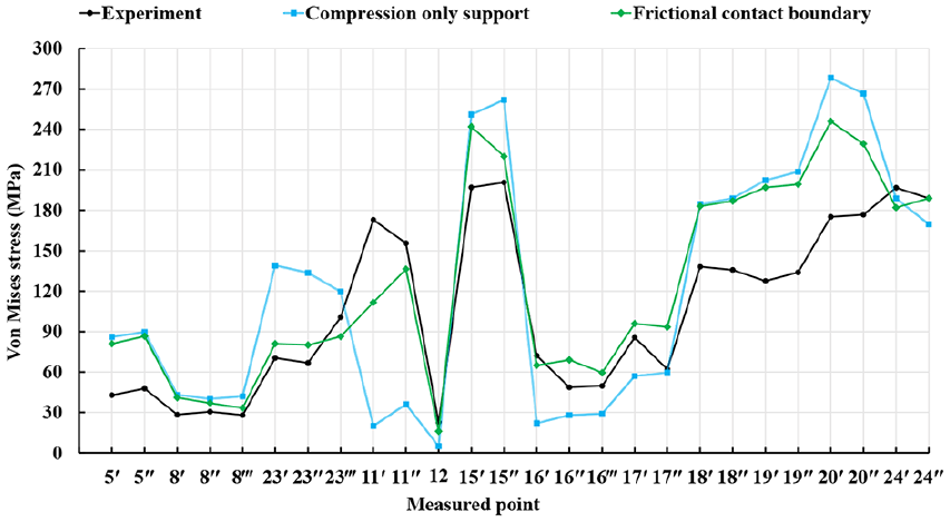
The comparison between the simulated and measured stresses is shown in Figure 9. The figure shows that the simulated stresses at the frictional contact boundary are closer to the measured stresses. However, the stress values of measured points in canopy and base are smaller than experimental results, and the simulated stress value of canopy is especially small. The possible reason is that the constraints of the canopy are excessive under the strength simulation of the above two conditions. The contact status and contact stresses of condition 3 and condition 4 under the frictional contact boundary are shown in Figure 10.

Figure 9.

Stress comparison: (a) condition 3 and (b) condition 4.

Figure 10.

Contact status and stress distributions under the friction contact boundaries: (a) condition 3 and (b) condition 4.

Adopting the same boundary constraint method as conditions 3 and 4, the comparison between the simulated and measured stresses of condition 5 is shown in Figure 11(a). The figure shows there exist large errors between the simulation and experiment and the simulated stresses are almost all less than the measured stresses except for measured points 24′ and 24′′. This shows the constraint generates a large local and whole stiffness which leads to a small deformation and stresses. In order to revise this deficiency, two short edges of two cushion blocks are fixed (see c₁ and c₂ lines in Figure 1(e)), and the contact between the cushion blocks and the base is set as the bonded contact. The contact between the canopy and the upper working table is set as the compression only support and the frictional contact, respectively. Under the revised boundary, the stress comparison is shown in Figure 11(b). The simulated stresses have a great improvement which agrees well with the measured stresses except for the canopy. The contact status and contact stress distributions also show that the boundary of the base has a slight influence on the frictional contact boundary, as is shown in Figure 12. The figure shows that the local contact phenomenon appears due to the concentrated load at socket positions. Due to the unevenness of the contact surface in real conditions, it is difficult to simulate the real experiment status by frictional contact boundary.

Figure 11.

Stress comparison at condition 5: (a) fixed constraint of bottom surfaces of two cushion blocks and (b) fixed constraint of short edges of two cushion blocks.

Figure 12.

Contact status and contact stress distributions under condition 5: (a) fixed constraint of bottom surfaces of two cushion blocks and (b) fixed constraint of short edges of two cushion blocks.

Elastic-support boundary conditions

The comparison results in Section 3.2.1 show that the frictional contact boundary can not accurately simulate the stress distribution of the canopy. It is found that there is a warping angle of about 2° between the front half and the rear half of the canopy. During the experiment, the canopy and the upper working table are not fully in contact at the beginning, but four points or lines around the canopy contact the upper working table first. With the increasing pressure load, the contact area will gradually increase.

By analyzing the actual condition characteristics, a new boundary condition is proposed to revise this deficiency (see Figure 13). Four corner points P₁, P₂, P₃, and P₄ on the canopy are fixed, and a spring constraint in Y-direction is added at the midpoint of line L₁ on the canopy. It should be noted that the Y-direction displacement of line L₂ is also constrained under condition 4 (see Figure 13(b)). The constraint of the bottom surfaces of cushion blocks and the contact between the upper surfaces of cushion blocks and the base are the same as those set in Section 3.2.1.

Figure 13.

Schematics of elastic support boundaries: (a) condition 3, (b) condition 4, and (c) condition 5.

Under three loading conditions, the effects of spring stiffness on the errors between the simulated and measured stresses are shown in Figure 14. It should be noted that spring stiffness “∞” denotes the Y-direction displacement of the line L₁ is constrained. Under condition 3, the error decreases first in the stiffness range of 0.1–1000 kN/mm and then increases in the stiffness range of 1000–∞ kN/mm. An optimal stiffness value can be determined as 1000 kN/mm (see Figure 14(a)). The optimal stiffness values for conditions 4 and 5 are about 100 and 5000 kN/mm, respectively (see Figure 14(b) and (c)).

Figure 14.

Stress errors comparison under different spring stiffness: (a) condition 3, (b) condition 4, and (c) condition 5.

The stress comparison under different spring stiffness is shown in Figure 15. The figure shows the spring stiffness has a great influence on the stress distribution of the canopy.

Figure 15.

Stress comparison: (a) condition 3, (b) condition 4, and (c) condition 5.

The stress nephograms under the frictional contact and elastic support boundaries (k = 1000, 50, and 5000 kN/mm for conditions 3, 4, and 5) are shown in Figure 16. The figure shows that the stress of the canopy is very small except for the socket positions in which the stress is about 50–100 MPa under the frictional contact boundary. When a reasonable elastic support boundary is adopted, the stress distribution is in good agreement with the experimental results.

Figure 16.

Comparison of stress nephograms: (a) condition 3, (b) condition 4, and (c) condition 5.

Stress comparison under the canopy eccentric loading condition (condition 2)

Compression only support and frictional contact boundary conditions

In this section, the boundary conditions between the base and the lower working table are set as frictional contact and compression only support, respectively. The contact between the cushion blocks and the canopy is set as bonded contact, and frictionless support boundary is applied to the upper surface of the cushion blocks.

The simulated stress results under the two boundaries are compared with the experimental results, as shown in Figure 17. The figure shows that the simulation result under the frictional contact boundary is closer to the experimental result than that under compression only support boundary. But there still exist large errors between the simulated and measured stresses at most measured points. The contact status shows that the local contact phenomenon is obvious due to the eccentric loading (see Figure 18).

Figure 17.

Stress comparison under condition 2.

Figure 18.

Contact status of base.

Elastic-support boundary conditions

According to the contact status, a proposed elastic-support boundary is established, the spring constraint is applied to the base of hydraulic support in Y-direction, and the fixed constraint is applied in X-direction and Z-direction, as is shown in Figure 19. In the figure, the left-side spring number and stiffness are larger than those at the right-side base, and k₁ = 10k₂.

Figure 19.

Schematic of elastic-support boundary under condition 2.

The effects of spring stiffness k₁ on the errors between simulated and measured stresses are shown in Figure 20(a), which indicates there exists a minimum error at k₁ = 200 kN/mm. The stress distributions at k₁ = 40, 200 kN/mm also show a similar trend as the experimental results (see Figure 20(b)). In summary, the total stiffness value of the right-side base is 1600 kN/mm (eight identical springs with stiffness of k₁), and the total stiffness value of the left-side base is 240 kN/mm (a spring with stiffness of k₁ and two springs with stiffness of k₂).

Figure 20.

(a) Stress error comparison and (b) stress comparison under different spring stiffness.

The upwarping angle phenomenon under the two boundary conditions is shown in Figure 21. It can be seen that Y-direction maximum displacement is 7.6 mm under the elastic-support boundary, which is smaller than 37.2 mm under the frictional contact boundary. It is clear that the larger deformation will result in the larger stress and this will cause the inaccuracy simulation result under the frictional contact boundary. The stress distribution under the elastic-support boundary is lower than that under the frictional contact boundary. The measured Y-direction maximum displacement is about 10–20 mm, which is closer to the simulated 7.6 mm. This also verifies the effectiveness of the elastic-support boundary.

Figure 21.

Local deformations (left figure) and stress distribution (right figure) under two boundaries: (a) frictional contact boundary and (b) elastic-support boundary.

Conclusions

The effects of the contact between the pin and shaft hole, and the boundary conditions on the stress distribution of hydraulic support are discussed based on the finite element simulation and experiment. Based on the experimental results, the reasonable pin-joint simplification and constraint boundaries are determined under five loading conditions. The main conclusions are summarized as follows:

The bonded contact and frictional contact between the pin and shaft hole all have a high accuracy, however, the former is more efficient. The bonded contact can be used as a better choice to evaluate the stress distribution of hydraulic support.

Traditional frictional contact boundary has a high accuracy under canopy torsional loading condition, however, there exist large errors at measured points on canopy or base due to the uneven phenomena (local contact phenomena) in the bottom surface of the base and top surface of the canopy. A new elastic-support boundary is proposed to revise this deficiency. The value range of elastic support stiffness is determined based on measured stress. For example, appropriate stiffness values are recommended such as 1000, 50, and 5000 kN/mm for base torsional, diagonal, and symmetrical loading conditions, respectively. For the canopy eccentric loading condition, the total stiffness value is 1600 kN/mm (eight identical springs with stiffness of the 200 kN/mm) at the right side of the base and it is 240 kN/mm (a spring with the stiffness of 200 kN/mm and two identical springs with the stiffness of 20 kN/mm) at the left side of the base.

Supplemental Material

sj-pdf-1-ade-10.1177_16878140211001194 – Supplemental material for Effects of boundary conditions on stress distribution of hydraulic support: A simulation and experimental study

Supplemental material, sj-pdf-1-ade-10.1177_16878140211001194 for Effects of boundary conditions on stress distribution of hydraulic support: A simulation and experimental study by Junzhe Lin, Tianrui Yang, Kaixuan Ni, Chenyi Han, Hui Ma, Ang Gao and Chunliang Xiao in Advances in Mechanical Engineering

Footnotes

Handling Editor: James Baldwin

Declaration of conflicting interests

The author(s) declared no potential conflicts of interest with respect to the research, authorship, and/or publication of this article.

Funding

The author(s) disclosed receipt of the following financial support for the research, authorship, and/or publication of this article: This project is supported by the National Natural Science Foundation (Grant nos. 11972112, 11772089), the Fundamental Research Funds for the Central Universities (Grant nos. N2003008, N2003014, and N180708009) and Liaoning Revitalization Talents Program (Grant No. XLYC1807008).

ORCID iD

Hui Ma

Supplemental material

Supplemental material for this article is available online.

References

Yang

Zeng

Zhou

, et al. The design and analysis of a new slipper-type hydraulic support. PLoS One 2018; 13: e0202431.

Xie

Wang

, et al. A virtual adjustment method and experimental study of the support attitude of hydraulic support groups in propulsion state. Measurement 2020; 158: 107743.

Liang

Fang

, et al. A fiber Bragg grating tilt sensor for posture monitoring of hydraulic supports in coal mine working face. Measurement 2019; 138: 305–313.

Zhang

Cao

Jiang

, et al. Simulation research on hydraulic support based virtual prototyping. In: 9th China-Russia symposium “Coal in the 21st century: mining, intelligent equipment and environment protection” (COAL 2018), Qingdao, China, 8–21 October 2018, pp.172–178. Paris: Atlantis Press.

Sun

Jiang

. Research on hydraulic-powered roof supports test problems. J Coal Sci Eng (China) 2011; 17: 201–206.

Wang

Yang

Feng

, et al. Stress analysis and stability analysis on doubly-telescopic prop of hydraulic support. Eng Fail Anal 2013; 32: 274–282.

Fan

. Analysis of the strength and reliability of hydraulic support with finite element method. Adv Mat Res 2013; 619: 225–230.

Zeng

Meng

Zhou

. Analysis on the pose and dynamic response of hydraulic support under dual impact loads. Int J Simul Model 2018; 17: 69–80.

Zeng

Meng

Zheng

. Force transmission analysis of sliding block-type hydraulic support under impact loads. Int J Simul Model 2019; 18: 100–111.

10.

Yang

Sun

Jiang

, et al. Structural analysis on impact-mechanical properties of ultra-high hydraulic support. Int J Simul Model 2020; 19: 17–28.

11.

Liao

Zhu

Keshtegar

, et al. Probabilistic framework for fatigue life assessment of notched components under size effects. Int J Mech Sci 2020; 181: 105685.

12.

Niu

Wang

Liao

, et al. Probabilistic modeling of uncertainties in fatigue reliability analysis of turbine bladed disks. Int J Fatigue 2021; 142: 105912.

13.

Zhu

Liao

, et al. The effect of notch size on critical distance and fatigue life predictions. Mater Des 2020; 196: 109095.

14.

Huangfu

Chen

, et al. Meshing and dynamic characteristics analysis of spalled gear systems: a theoretical and experimental study. Mech Syst Signal Process 2020; 139: 106640.

15.

Chen

Huangfu

, et al. Calculation of mesh stiffness of spur gears considering complex foundation types and crack propagation paths. Mech Syst Signal Process 2019; 130: 273–292.

16.

Gohari

Sharifi

Sharifishourabi

, et al. Effect of temperature on crack initiation in gas formed structures. J Mech Sci Technol 2013; 27: 3745–3754.

17.

Gohari

Sharifi

Burvill

, et al. Localized failure analysis of internally pressurized laminated ellipsoidal woven GFRP composite domes: analytical, numerical, and experimental studies. Arch Civ Mech Eng 2019; 19: 1235–1250.

18.

Hong

, et al. Strength analysis of hydraulic support under multi working conditions and multi height. Colliery Mech Electr Technol 1992; 2: 11–14.

19.

, et al. Strength finite element analysis of hydraulic powered support based on ANSYS. Coal Mine Mach 2006; 27: 91–93.

20.

Gou

Lei

, et al. Strength analysis of mine hydraulic support. J Chongqing Univ Technol (Nat Sci) 2014; 28: 44–47.

21.

Gao

Zhou

. Simulation of strength test of hydraulic support by means of finite element method. J Mech Des 2018; 35: 66–71.

22.

. Comparative analysis of stress tests of certain type hydraulic support. Coal Technol 2015; 34: 244–246.

23.

Xie

Qin

. Strength and reliability analysis of hydraulic support. Adv Mat Res 2012; 544: 18–23.

24.

Xie

Hong

, et al. Finite element analysis and hydraulic support stress test. Mach Des Manuf 2012; 11: 34–36.

25.

Liu

. Hydraulic support entire strength research under four kinds of typical load working conditions. In: Second international conference on mechanic automation and control engineering, Inner Mongolia, China, 15–17 July 2011, pp.329–332. New York: IEEE.

26.

Zheng

. Three-dimensional modeling and finite element analysis of the hydraulic support. Adv Mat Res 2013; 712–715: 1002–1005.

27.

Zhao

Liu

, et al. Fatigue behavior of a box-type welded structure of hydraulic support used in coal mine. Materials 2015; 8: 6609–6662.

28.

Feng

Tang

. Strength analysis of six-pillar hydraulic support base. In: Zhang

Wei

(eds) Mechanics and architectural design. Singapore: World Scientific Publishing, 2017, pp.61–71.

29.

Kong

Wang

. The strength adaptability analysis of super-large mining height hydraulic support. Int Core J Eng 2017; 3: 229–237.

30.

GB 25974.1-2010. Powered support for coal mine part 1: general specification. The State Standard of the People’s Republic of China, 2011.

31.

Zhu

. Stress research and finite element analysis of hydraulic support. Master’s Thesis, Northeastern University, USA, 2011.

Supplementary Material

Please find the following supplemental material available below.

For Open Access articles published under a Creative Commons License, all supplemental material carries the same license as the article it is associated with.

For non-Open Access articles published, all supplemental material carries a non-exclusive license, and permission requests for re-use of supplemental material or any part of supplemental material shall be sent directly to the copyright owner as specified in the copyright notice associated with the article.

0.00 MB

0.02 MB