
Abstract
The objective of this research was to investigate the effects of material models, element types, and boundary conditions on the consistency of finite element analysis. Two cantilever beams were used; one made of stainless steel SUS301 3/4H and the other made of polymer polyoxymethylene. The load–deflection curves of the two cantilever beams obtained by experiments were compared to those obtained by finite element analysis, where the material models—including bilinear, trilinear, and multi-linear—were used. Four element types—beam, plane stress, shell, and solid—were also employed with the material models to obtain the simulated load–deflection curves of the cantilever beams. It was found that bilinear material models had the stiffest behavior due to their overestimated yield strength. In addition, by applying a finite displacement to simulate the grip of the cantilever beams, the discrepancy between the simulated permanent set and the experimental set could be reduced from 80% to 5%. To sum up, both the selection of the material model and the setup of the boundary conditions are critical for obtaining good agreement between the finite element analysis results and the experimental data.
Introduction
Accuracy is usually a concern when performing finite element analysis (FEA). In actual engineering applications, there are usually no analytical solutions available. Those not familiar with FEA may expect that the analysis results should be as close to the experimental results as possible, implicitly assume that the experimental data are error-free, and can be used for determining the accuracy of the FEA results. However, this assumption is not true, as measurement in experiments always contains errors, which may be introduced by the operators or the measuring equipment. However, analysis results also contain errors, which include formulation errors, discretization errors, and round-off errors. By comparing these possible errors with the experimental data, it may be reasonable to assume that the deviations between the experimental data and the exact results are small so that the experimental data can be used as a reference for computational consistency. Also, the uncertainties due to the geometric tolerances, material parameters, and boundary conditions may also contribute to the variation of the finite element solution. 1 Commercial FEA software packages usually allow users to define the material model, adjust the mesh density, and choose the element type because they are all related to the accuracy of the results. 2 However, how to choose the proper settings so that analysis results can be efficiently obtained, and with reasonable consistency, remains a challenge for many FEA users.
A previous study by Cifuentes and Kalbag 3 demonstrated that the quadratic tetrahedral element might behave as well as the quadratic hexagonal elements regarding accuracy and CPU time. Li et al. 4 also reported that both tetrahedral element and hexahedral elements were valid by comparing the simulation results with the experimental data of a bogie frame. However, it was found that the hybrid hexahedral element performed well, but the hybrid tetrahedral element performed poorly for the simulation of the foot and footwear under compression and shear loading. 5 Muccini et al. 6 also showed that the linear tetrahedral element should be avoided during contact analysis due to its accuracy problem. Regarding the mesh density, Langer et al. 7 provided some guidelines for meshing: it was reported that at least 20 quadratic or 500 linear elements per standing wave were needed to achieve a solution for eigenfrequencies with an error of less than 1%.
However, Shi and Liu 8 studied different material models, such as those of Litonski–Batra, the power law, Johnson–Cook, and Bodner–Partom, for simulating orthogonal machining on an HY100 alloy. While some material models could generate accurate predictions of cutting force and chip formation, they failed to predict the residual stress. From their study, it seemed difficult to find one material model that could accurately predict behavior in all aspects of interest. Lăzărescu et al. 9 also used several constitutive models to generate yield surfaces for AA6016T4 aluminum alloy. Through hydraulic bulge testing, they found that, to obtain good agreement between the simulation and experimental data, the constitutive model BBC2005 with all the input parameters should be used. Thomas et al. 10 applied a cyclic loading using a punch on a simply supported circular plate to study various work hardening material models, including isotropic, kinematic, mechanical sublayer, and Mroz. They found that the mechanical sublayer model was the most efficient, and had good correlation with the experimental results. Amy et al. 11 presented various error sources while performing FEA, including material variability, dimensional tolerances, and input parameter inaccuracy. They also reported that the boundary condition was critical to the accuracy of the FEA.
In this study, the measurement data were employed as a reference to compare with the FEA results. As mentioned previously, the material model, the mesh density, and the element selection are critical factors that can affect consistency. Nevertheless, mesh density can be determined by observing the convergence of the solution with different mesh densities, so its effect was not considered here. The objective of this research was to find the effects of the material model, the element type, and the setup of the boundary condition on the consistency of the FEA results with respect to the measured results. Instead of using various constitutive equations for the material models, bilinear, trilinear, and multi-linear models were used. The conclusions drawn from this study can be used to improve consistency in future FEA.
Materials and methods
Material models
The materials used in this study were polyoxymethylene (POM), and stainless steel SUS301 3/4H. Tensile tests were performed to obtain the stress–strain curves of these two materials, and then, the curves were used to generate their material models to for use in FEA. To perform the tensile tests, POM specimens and SUS301 3/4H specimens were prepared according to ASTM D638 (Type I) and ASTM A370 (sheet type), respectively, and three specimens of each material were tested using a universal testing system (Instron 3365, Instron, MA, USA). The stress–strain curves of POM and SUS301 3/4H were obtained as shown in Figures 1 and 2, respectively. Please note that the stresses and strains used in this paper all refer to true stresses and true strains.

Experimental stress–strain curves and three material models for POM.

Experimental stress–strain curves and three material models for SUS301 3/4H.
In FEA, three material models were used: bilinear, trilinear, and multi-linear. These three models are commonly used when the material’s nonlinearity is considered. The POM models are illustrated in Figure 1, and those of SUS301 3/4H are illustrated in Figure 2. The bilinear material models were constructed by extending the linear portions in both the elastic region and the plastic region. The point where the two linear portions meet is the yield point for the bilinear material models. Young’s moduli, yield strengths, and tangent moduli of both the POM and SUS301 3/4H are listed in Table 1.
Parameters of bilinear material models of POM and SUS301 3/4H.

POM: polyoxymethylene.
To better describe the stress–strain curves of the POM and SUS301 3/4H, the trilinear material model, as shown in Figures 1 and 2, was used to represent the stress–strain relationship between the POM and SUS301 3/4H. Each trilinear model includes three linear portions: the first line and third line are the linear portions in the elastic region and plastic region, and the middle one is obtained by simply connecting the other two linear portions together. As shown in Figures 1 and 2, the yield points of the trilinear models are the points where the material starts to yield or the points where the first linear portions end. By comparing the yield points with those of the bilinear models, the yield points of the trilinear models are obviously lower. The stresses and strains used to define the trilinear material models of POM and SUS301 3/4H are listed in Table 2.
Parameters of trilinear material models of POM and SUS301 3/4H.

POM: polyoxymethylene.
The multi-linear material models of POM and SUS301 3/4H are also shown in Figures 1 and 2, respectively. Obviously, the material models best fit the experimental stress–strain curves. The stresses and strains used to define the multi-linear models can be found in Table 3, in which eight data points are used to construct each of the material models.
Parameters of multi-linear material models of POM and SUS301 3/4H.

POM: polyoxymethylene.
Methods
In this study, the comparison between the experimental data and the FEA results was made to determine consistency. The experiment was to apply loads to cantilever beams made of POM and SUS301 3/4H to obtain the load–deflection relationship. The size of the POM cantilever beam was 60.0 × 12.0 × 3.0 mm and that of the SUS301 3/4H beam was 30.0 × 8.0 × 0.4 mm. The actual lengths of the cantilever specimens were longer than the specified dimensions, as an extra length was needed for gripping. The experiments were conducted on the same universal testing system used to obtain the stress–strain curves of the materials. The horizontal cantilever beam specimens were clamped on the fixture, and then, a rack containing weights was loaded near the free end of the cantilever so that the load direction was always perpendicular to the ground, thus, simulating the fixed loading direction in FEA. The small unloaded portion of the cantilever beam was not included in the length of the cantilever beam so that it did not affect the simulation. The weights in the rack were gradually increased to obtain the load–deflection curves for the cantilever beams; the maximum loads were 15.5 N for POM and 10.6 N for SUS301 3/4H. Three cantilever beams were tested for each material, and the mean values were calculated to produce the load–deflection curves.
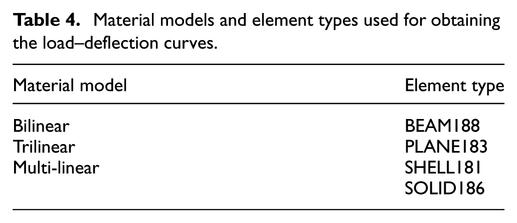
To obtain the analysis results, commercial FEA software ANSYS (Ansys Inc., Canonsburg, PA, USA) was used to perform the simulation. Table 4 lists the three material models and the four element types adopted in analysis. The four element types were BEAM188, PLANE183, SHELL181, and SOLID186. BEAM188 is a one-dimensional beam element, PLANE183 is a two-dimensional plane-stress quadrilateral element, SHELL181 is a three-dimensional shell quadrilateral element, and SOLID186 is a three-dimensional solid hexagonal element. All the elements were quadratic, meaning that there is a node in the middle of each edge of the elements. The boundary conditions, fixed support at the fixed end and a load at the free end, were applied to the finite element model to obtain the simulated load–deflection curves.
Material models and element types used for obtaining the load–deflection curves.
Results and discussion
Before the FEA was conducted on the cantilever beams, convergence tests were performed for all of the element types used in this study to determine the proper element sizes. It was found that the von Mises stresses of the cantilever beams converged when the element size was reduced to 1 mm for POM and 0.2 mm for SUS301 3/4H, respectively. Therefore, in subsequent analysis, these element sizes were used for the finite element models. The FEA results are presented by the materials in the following sections.
POM
The solid lines with various colors in Figure 3 represent the POM cantilever beam’s load–deflection curves, as obtained using the following elements: BEAM188, PLANE183, SHELL181, and SOLID186, respectively. The material model used to obtain the curves was bilinear. While Figure 3 shows that the calculated maximum deflections ranged from 19.5 to 20.8 mm, the actual maximum deflection was 24.64 mm. Apparently, the calculated results all underestimated the actual deflection. It was also found that the calculated POM’s permanent deflections were all trivial, and the actual one was 2.72 mm. The deviations in the calculated results from the experimental data are summarized in Table 5, in which both the values and the percentages are presented. It can be seen that the deviation percentage of the maximum deflection ranges from −16% to −21% and that of the permanent set ranges from −90% to −100%. Here, the negative sign indicates that the calculated results underestimated the measured data.

Actual load–deflection curve of the POM cantilever beam and the simulated ones with the use of various elements and a bilinear material model.
Deviations in the maximum deflection and the permanent set based on POM’s bilinear material model for various element types (the values in the parentheses indicate the deviations in percentage with respect to the experimental data).
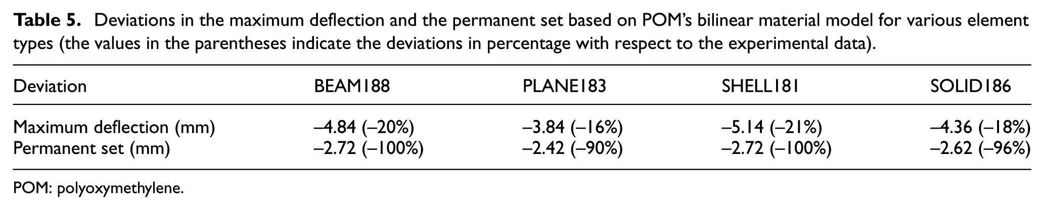
POM: polyoxymethylene.
To understand the cause of the significant deviation, Figure 1 shows that, while the bilinear model had a yield strength of 54.7 MPa, the POM started to yield at 26.1 MPa. This difference was one of the reasons that there were noticeable deviations, especially for the permanent set, between the calculated results and the simulated ones. Regarding element type, all four element types, BEAM188, PLANE183, SHELL181, and SOLID186, behaved similarly.
Then, the trilinear model, which better describes the nonlinear behavior of POM, was used to improve the consistency of the cantilever beam FEA. The analysis results of the POM cantilever beam are shown in Figure 4. Table 6 lists deviations at the maximum deflection, which ranged from 2% to 10% for the four element types used in this research. The deviations of the maximum deflection, as based on the trilinear model, are obviously less than those based on the bilinear model, which was due to the lower yield strength of the trilinear model, as depicted in Figure 1. Contrary to the results of the bilinear model, all the load–deflection curves of the trilinear material model overestimated the maximum deflection and permanent set. The deviations of the permanent set ranged from 163% to 218% as listed in Table 6. As mentioned previously, the yield strength of the trilinear model is less than that of the bilinear model; therefore, both the maximum deflections and the permanent sets, as calculated based on this trilinear model, were greater than those obtained for the bilinear case. Regarding the element types, BEAM188 and PLANE183 behaved similarly, as did SHELL181 and SOLID186.

Actual load–deflection curve of the POM cantilever beam and the simulated ones using various elements and a trilinear material model.
Deviations in the maximum deflection and the permanent set based on POM’s trilinear material model for various element types (the values in parentheses indicate deviations in percentage with respect to the experimental data).

POM: polyoxymethylene.
To continue to improve consistency, the multi-linear model was used to simulate the POM cantilever beam. Figure 5 shows the load–deflection curves obtained from the experiment and the FEA, as based on the four element types. In comparison with Figures 3 and 4, it can be seen that, for the same element type, the curve in Figure 5 is between those shown in Figures 3 and 4 as expected, because the stress–strain curve of the multi-linear model is also between those of the bilinear and trilinear models, as shown in Figure 1. Table 7 lists the deviations at the maximum deflection ranging from −6% to −14%, which are between the maximum deflections calculated using the bilinear and trilinear material models. The same situation occurred for the permanent set, which ranged from −21% to 15%. Regarding the element type, all four element types behaved differently.

Actual load–deflection curve of the POM cantilever beam and the simulated ones using various elements and a multi-linear material model.
Deviations in the maximum deflection and the permanent set based on POM’s multi-linear material model for various element types (the values in parentheses indicate deviations in percentage with respect to the experimental data).

POM: polyoxymethylene.
SUS301 3/4H
This study extended this section to another material, SUS301 3/4H, which used the same approach as the POM material. Regarding the SUS301 3/4H bilinear model, the results were similar to those of the bilinear model for POM. Figure 6 shows the load–deflection curves obtained using the experiment and finite element models, as based on the four element types. The deviations in the maximum deflections calculated using FEA with the four element types ranged from −6% to −11%, as indicated in Table 8. While the permanent sets calculated by FEA were trivial, the actual permanent set was 2.86 mm. This significant deviation was mainly due to the overestimated yield strength of the bilinear material model, as previously explained. Regarding the element type, all four element types, BEAM188, PLANE183, SHELL181, and SOLID186, behaved similarly.

Actual load–deflection curve of the SUS301 3/4H cantilever beam and the simulated ones using various elements and a bilinear material model.
Deviations in maximum deflection and the permanent set based on SUS301 3/4H’s bilinear material model for various element types (the values in parentheses indicate deviations in percentage with respect to the experimental data).

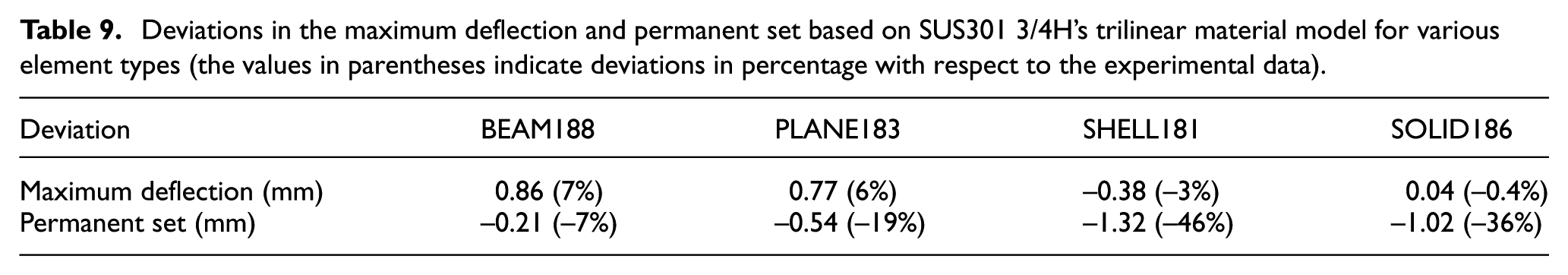
Then, the trilinear model was used to calculate the deflection and permanent set of the cantilever beam, and Figure 7 illustrates the results. The deviations in the calculated maximum deflections, as listed in Table 9, ranged from −0.4% to 7%, which were quite consistent with the experimental maximum deflection. Next, the deviations in the permanent set calculation ranged from −7% to −46%, as indicated in Table 9. Compared to results of the POM case, as listed in Table 6, the calculated permanent sets based on the trilinear model for SUS301 3/4H were relatively consistent with the experimental results. Regarding the element types, BEAM188 and PLANE183 behaved similarly, as did SHELL181 and SOLID186.

Actual load–deflection curve of the SUS301 3/4H cantilever beam and the simulated ones using various elements and a trilinear material model.
Deviations in the maximum deflection and permanent set based on SUS301 3/4H’s trilinear material model for various element types (the values in parentheses indicate deviations in percentage with respect to the experimental data).
Finally, using the multi-linear material model for SUS301 3/4H, the load–deflection curves were obtained, as shown in Figure 8. As the multi-linear model is stiffer than the trilinear model, as illustrated in Figure 2, the load–deflection curves in Figure 8 shifted to the left, as compared to the curves in Figure 7. This trend was similar to that of the POM case. The deviations at the maximum deflection, using the four element types, ranged from −1% to −8%, while the deviations of the permanent set ranged from −62% to −77%, as indicated in Table 10. Regarding the element types, BEAM188 and PLANE183 behaved similarly, as did SHELL181 and SOLID186. While the deviations in the maximum deflection between the calculated and the experimental results seemed to be small, those of the permanent set between the calculated and the experimental results were large, which may indicate that there was an unknown factor that affected the results of the permanent set.

Actual load–deflection curve of the SUS301 3/4H cantilever beam and the simulated ones using various elements and a multi-linear material model.
Deviations in the maximum deflection and the permanent set based on SUS301 3/4H’s multi-linear material model for various element types (the values in parentheses indicate deviations in percentage with respect to the experimental data).

One possible factor was the stress caused by the grip. In the cantilever beam experiment, a portion of the cantilever was firmly gripped to provide support. The stresses of the specimens at the grip were generated, which may have contributed to the large permanent set in the SUS301 3/4H’s case. Regarding simulation, we simply used boundary conditions with gripping portions permanently fixed at the initial position; thus, there were no stresses at the grip. To reduce the deviation in the boundary conditions between the experiment and the simulation, further simulations were performed using the modified boundary condition, as discussed in the following.
Study on the setup of the boundary condition
In this section, a cantilever beam made of another material, SUS301 H, was analyzed to examine the setup of the boundary condition. The size of the beam was the same as the one made of SUS301 3/4H, and the procedure was similar to that presented in the previous sections. First, the specimens were made using the SUS301 H material. Next, tensile testing was performed to obtain the stress–strain curve to build the multi-linear material model. Then, FEA, as based on the multi-linear material model, was performed with boundary conditions with and without pre-stress to obtain results. Pre-stress was generated by assigning a downward displacement on top of the gripping area, as shown in Figure 9, to simulate the stress created due to the grip on the specimen. Only the SOLID186 element type was used for this study, as BEAM188 and SHELL181 cannot be applied to the finite displacement boundary condition. PLANE183, which is a two-dimensional element type, cannot be used for the general three-dimensional structure as well.

Pre-stress boundary conditions of the SUS301 H cantilever beam.
Regarding the boundary condition without pre-stress, the calculated deflection at the maximum load was 11.15 mm, which was 1.85 mm or 14% less than the experimental results, as indicated in Table 11, while the calculated permanent set was 2.55 mm or 80% less than the experimental data. Obviously, the simulation results were not consistent with the experimental data, especially for the permanent set. Regarding the boundary condition with pre-stress, the calculated deflection at the maximum load was 0.03 mm or 0.2% less than the experimental data, while the calculated permanent set was 0.15 mm or 5% more than the experimental data. The simulated results with pre-stress greatly improved the consistency. Here, the press-stress was simulated based on the displacement of 0.2 mm, which was measured during the experimental setup.
Comparison of the deviations for SUS301 H by FEA with the use of SOLID186 element (pre-stress at displacement 0.02 mm).
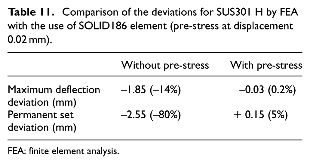
FEA: finite element analysis.
The stresses created by the grip increased the stress at the fixed end of the cantilever beam did affect the simulated results. If the stresses are ignored, a significant deviation of the permanent set may occur. If the stresses are included in FEA by imposing displacement at the grip, then, how to determine the displacement becomes a critical issue. The analysis process found that the permanent set was very sensitive to the value of displacement. In a real situation, FEA analysts may have difficulty setting up this displacement boundary condition unless the experimental data are available. Without properly setting up the boundary conditions according to the actual boundary conditions of the experiment, inconsistency between the simulated results and the experimental data is expected.
Conclusive remarks
FEA software has proven to be an indispensable tool for researchers and engineers in solving engineering problems. The objective of this research was to study and improve the consistency of FEA using various element types, material models, and the setup of the boundary conditions. The four element types used in this research were BEAM188, PLANE183, SHELL181, and SOLID186. Three material models—the bilinear model, trilinear model, and multi-linear model—were used to simulate the behavior of cantilever beams made of both POM and SUS301 3/4H. The study findings are summarized as follows. When the stress–strain curve of the materials is not available for finite element simulation, to use limited information such as yield strength, Young’s modulus, and tangent modulus, to create an approximate stress–strain curve as a bilinear curve may be inappropriate. The yield strength of the bilinear stress–strain curve may be much higher than that of the actual stress–strain curve, which may result in less deflection and permanent set. To use the trilinear or the multi-linear stress–strain curve is a better choice in adopting the material model. In addition, the deviation between the FEA results and the experimental results may be due to the over-simplified boundary condition setup. Simply fixing the displacement of the boundary without considering the stresses induced by the grip may underestimate the permanent set generated at the boundary.
Footnotes
Handling Editor: Artde Lin
Declaration of conflicting interests
The author(s) declared no potential conflicts of interest with respect to the research, authorship, and/or publication of this article.
Funding
The author(s) disclosed receipt of the following financial support for the research, authorship, and/or publication of this article: The authors thank the Ministry of Science and Technology, Republic of China, for the financial support of this research under grant MOST 105-2221-E-011-055.