Optimization of the setup position of a workpiece for five-axis machining to reduce machining time

Abstract

Five-axis machining is commonly used for complicated features due to its advantage of rotary movement. However, the rotary movement introduces nonlinear terms in the kinematic transform. The nonlinear terms are related to the distance between the cutter location (CL) data and the intersection of the two rotary axes. This research studied the possible setup positions after the toolpaths have been generated, and the objective was to determine the optimal setup position of a workpiece with minimal axial movements to reduce the machining time. We derived the kinematic transform for each type of five-axis machines, and then, defined an optimization problem that described the relationship between the workpiece setup position and the pseudo-distance of the axial movements. Eventually, an optimization algorithm was proposed to search for the optimal workpiece setup position within the machinable domain, which is already concerned with over-traveling and machine interference problems. In the end, we verified the optimal results with a case study with a channel feature, which was real cutting on a table-table type five-axis machine. The results show that we can save the axial movements up to 16.76% and the machining time up to 10.70% by setting up the part at the optimal position.

Introduction

Background

In general, a five-axis machine is constructed with three linear axes and two rotary axes, with which the cutting tool can be tilted to cut free-form surfaces and avoid collision between the tool and the workpiece. In addition, the workpiece can be fabricated within minimum setup times, which can effectively reduce machining time including the time for planning multiple setups and making customized fixtures. Although the five-axis machining has the advantages mentioned above, it still requires operators to make many decisions, such as tool selection, tool orientation, and setup position, which may affect the machining efficiency.

Usually, engineers could directly generate the five-axis toolpaths for a part using CAM software. The toolpaths represent the tooltip position and the tool orientation, based on the workpiece coordinate system (WCS). Nevertheless, the machine only recognizes the position relative to the machine coordinate system (MCS). Thus, a transformation between the WCS and the MCS is necessary. During the process, the tool trajectory is complex due to the motion caused by the two rotary movements. Moreover, due to the varying distance between the tooltip position and the rotary center, different setup positions can cause different tool trajectories in MCS. In other words, machining efficiency can be improved by optimizing the setup position of a workpiece. Until now, the decision for a setup position still depends on the operator’s experience. The experience cannot guarantee that the two major issues will not occur: one is the collision between the tool assembly and the machine components, and the other is over-traveling occurring on the linear axes. Additionally, little research on the relationship between the setup position and the machining efficiency has been made.

Literature review

In general, cutter location (CL) data is used to describe the toolpaths. The CL data have to be transformed to the NC code, which is based on the MCS, so that the machine can move accordingly. Thus, the kinematic transforms for five-axis machine structures are needed. Five-axis machine are commonly categorized into three types: head-head, head-table, and table-table, based on the location of the two rotary axes. Many researchers have studied kinematics of the machines using the homogeneous coordinate transformation matrices in Denavit-Hartenberg notation. ¹ Lee and She ² derived kinematics for a head-head type, a head-table type, and a table-table type. Jung et al. ³ developed a postprocessor for a table-table five-axis machine tool with A and C axes (TATC), and then proposed an algorithm to prevent interference in certain situations. She and Lee ⁴ and She and Chang ⁵ designed a generalized kinematic model, which combines the primary and the secondary rotary axes on both the spindle side and the table side. The generalized kinematic model can be applied to all types of five-axis machine tools. Sørby ⁶ derived forward and inverse kinematics for five-axis machine tools with non-orthogonal rotary axes B and C on the worktable. Yang and Altintas ⁷ used the screw theory to develop a generalized forward and inverse kinematic transform method, which models each kinematic element as a revolute joint or prismatic joint. The screw theory method can easily calculate the inverse kinematics with only the point and vector of each joint. Many researchers developed kinematic models containing nonlinear terms due to the involvement of two rotary axes. The nonlinear terms result in variations of distance equation within five-axis machining trajectories. The result of distance equation could be altered in two aspects, as discussed in the following. One is the orientation of the workpiece; the other is the position of the workpiece. However, the two factors are too complicated to be considered at the same time. Some researchers studied the effects of the orientation of a workpiece on planning the toolpath. Lee et al. ⁸ determined the optimal workpiece orientation by the minimum rotary movement. Hu et al. ⁹ determined the optimal setup by the largest intersection of the visibility maps. Some researchers studied the position of the workpiece after the toolpath had been defined. Anotaipaiboon et al. ¹⁰ studied the optimization problem of the workpiece position to minimize the kinematic errors caused by nonlinear tool trajectory. Tutunea-Fatan and Bhuiya ¹¹ proposed a method to determine the nonlinear errors of the head-head type five-axis machine. Then, they compared the efficiency between the structures with different combinations of rotary axes, and found that the combination with vertical rotational axis tends to move more than with only horizontal rotational axes. Lin et al. ¹² focused on the movement errors on a TATC type machine. Then, the optimal workpiece position was found by using particle swarm optimization in the machinable domain to minimize the nonlinear error caused by the rotary movement. The machinable domain was constructed as a cuboid field according to the travel of three linear axes of machine. Xu and Tang ¹³ considered energy efficiency on the movement of each axis. Then, they proposed an algorithm to find the optimal workpiece setup with minimum energy cost. Shaw and Ou ¹⁴ derived a transformation matrix on a TATC type machine to find the minimum movement on the X, Y, and Z axes. Then, he used a generic algorithm to search for the best position for the workpiece in a cuboid domain that formed with a limit of three linear axes. Pessoles et al. ¹⁵ defined the pseudo-distance as a sum of the maximum movement for the three linear axes along the toolpaths. He discretized the possible domain of a workpiece setup position, and then he computed the pseudo-distances for all the setup positions. Eventually, the optimal workpiece setup position was determined by finding the minimum pseudo-distance.

Objective

The research above studied about the machining distance of table-table type machines with AC type and BC type configurations. Nevertheless, the relationship between the workpiece position and the machining time is still unknown for different types of five-axis machines. The machining time is a complicated issue affected by system performance, including toolpath trajectory complexity, acceleration planning, and motor response. To simplify the problem, we considered the axial movement distance as a measure of the machining time and ignored all the other factors that may affect the machining time. In addition, over-traveling and interference problems between the tool assembly and the machine components have not been considered yet. In other words, the workpiece may not be completed due to over-traveling or interference problems. Therefore, the objective of this research was to determine the optimal setup position of a workpiece with minimal axial movements on a tool trajectory in a machinable domain, where the workpiece can be machined with one setup without problems including over-traveling of each axis or interference between the tool assembly and the machine components.

Statement of the optimization problem

Kinematics of a five-axis machine ¹⁶

In this section, we only derived the kinematic transform of A and C rotary axes for each type of the machines. Likewise, the machine with different rotary axes can be derived. To derive the kinematic model for each type of five-axis machine, we have to use six coordinate systems: WCS (O_WXYZ) and MCS (O_MXYZ) and the other four are defined as follows.

1. The coordinate system at the fourth rotary center (O₄XYZ), which is the center of the primary rotary axis.

2. The coordinate system at the fifth rotary center (O₅XYZ), which is the center of the second rotary axis.

3. The spindle-nose coordinate system (SCS, O_SXYZ), which is located at the center of the spindle-nose.

4. The tool coordinate system (TCS, O_TXYZ), which is located at the controlled cutting point on the tool. The cutting point can be either the tooltip or the tool center.

The relationship between the six coordinate systems in a TATC type, which means the fourth axis is an A axis, and the fifth axis is a C axis on a table-table type five-axis machine, can be illustrated in Figure 1. As shown in the figure, ${\mathbf{d}}_{\mathbf{M}\to \mathbf{S}}$ represents the vector from O_MXYZ to O_SXYZ; ${\mathbf{d}}_{\mathbf{S}\to \mathbf{T}}$ represents the vector from O_SXYZ to O_TXYZ; ${\mathbf{d}}_{\mathbf{M}\to 4^{\mathbf{th}}}$ represents the vector from O_MXYZ to O₄XYZ; ${\mathbf{d}}_{4^{\mathbf{th}}\to 5^{\mathbf{th}}}$ represents the vector from O₄XYZ to O₅XYZ; ${\mathbf{d}}_{5^{\mathbf{th}}\to \mathbf{W}}$ represents the vector from O₅XYZ to O_WXYZ.

Figure 1.

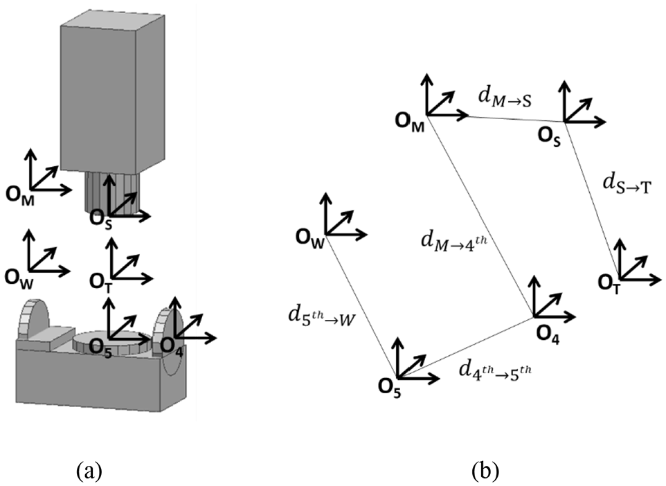
(a) Coordinate systems defined on the table-table type five-axis machine and (b) their relationship.

The CL data can be transformed from O_WXYZ to O_MXYZ in five steps. The overall transformation matrix on the table side can be obtained through the five steps described below:

1. Translate from O_WXYZ to O₅XYZ with vector ${\mathbf{d}}_{5^{\mathbf{th}}\to \mathbf{W}}$ .

2. Rotate an angle $-C$ around the C axis in O₅XYZ.

3. Translate from O₅XYZ to O₄XYZ with vector ${\mathbf{d}}_{4^{\mathbf{th}}\to 5^{\mathbf{th}}}$ .

4. Rotate an angle $-A$ around the A axis in O₄XYZ.

5. Translate from O₄XYZ to O_MXYZ with vector ${\mathbf{d}}_{\mathbf{M}\to 4^{\mathbf{th}}}$ .

We define $\mathbf{Trans}(\mathbf{d})$ as a translation transformation matrix with vector $\mathbf{d}$ , and $\mathbf{RotX}(A)$ , $\mathbf{RotY}(B)$ , $\mathbf{RotZ}(C)$ as a rotary transformation matrix with A, B and C angles rotated around the X, Y, and Z axes, respectively. In this case, the rotary axis is placed on the table side. Since the direction of rotary movement is defined by the tool, the rotary direction is opposite when the rotary axis is on the table side. After all the transformations are performed, the cutter location can be represented in O_MXYZ. To coincide the controlled cutting point on the tool to the cutter location in terms of the MCS, we need to transform the position of the cutting point from O_TXYZ to O_MXYZ. The transformation matrix of the spindle side, which is denoted by the matrix $\mathbf{S}$ , can be derived in two steps: (1) Translate from O_SXYZ to O_TXYZ with vector $\mathbf{t}$ , which is defined as the vector from the cutting location on the tool to the spindle-nose. (2) Translate from O_MXYZ to O_SXYZ with vector ${\mathbf{d}}_{\mathbf{M}\to \mathbf{S}}$ . Thus, the two transformation matrices of the TATC machine are defined as equations (1) and (2).

• (1) TATC type

$$\begin{array}{c}\multicolumn{1}{c}{\mathbf{T}=\mathbf{Trans}({\mathbf{d}}_{\mathbf{M}\to 4^{\mathbf{th}}})·\mathbf{RotX}(-A)·\mathbf{Trans}({\mathbf{d}}_{4^{\mathbf{th}}\to 5^{\mathbf{th}}})·}\\ \mathbf{RotZ}(-C)·\mathbf{Trans}({\mathbf{d}}_{5^{\mathbf{th}}\to \mathbf{W}})\hfill \end{array}$$

(1)

$$\mathbf{S}=\mathbf{Trans}({\mathbf{d}}_{\mathbf{M}\to \mathbf{S}})·\mathbf{Trans}({\mathbf{d}}_{\mathbf{S}\to \mathbf{T}})$$

(2)

Similarly, the relationship between each coordinate system of the head-table type and head-head type, or the HATC type and the HCHA type, five-axis machine can be illustrated in Figures 2 and 3, respectively. The transformation of these two types of machines can be derived by using the kinematic chain loop as well. The transformation matrices are defined as equations (3) to (6).

• (2) HATC type

$$\mathbf{T}=\mathbf{Trans}({\mathbf{d}}_{\mathbf{M}\to 5^{\mathbf{th}}})·\mathbf{RotZ}(-C)·\mathbf{Trans}({\mathbf{d}}_{5^{\mathbf{th}}\to \mathbf{W}})$$

(3)

$$\mathbf{S}=\mathbf{Trans}({\mathbf{d}}_{\mathbf{M}\to 4^{\mathbf{th}}})·\mathbf{RotX}(A)·\mathbf{Trans}({\mathbf{d}}_{4^{\mathbf{th}}\to \mathbf{S}})·\mathbf{Trans}({\mathbf{d}}_{\mathbf{S}\to \mathbf{T}})$$

(4)

• (3) HCHA type

$$\mathbf{T}=\mathbf{Trans}({\mathbf{d}}_{\mathbf{M}\to \mathbf{W}})$$

(5)

$$\begin{array}{c}\multicolumn{1}{c}{\mathbf{S}=\mathbf{Trans}({\mathbf{d}}_{\mathbf{M}\to 4^{\mathbf{th}}})·\mathbf{RotZ}(C)·\mathbf{Trans}({\mathbf{d}}_{4^{\mathbf{th}}\to 5^{\mathbf{th}}})·}\\ \mathbf{RotX}(A)·\mathbf{Trans}({\mathbf{d}}_{5^{\mathbf{th}}\to \mathbf{S}})·\mathbf{Trans}({\mathbf{d}}_{\mathbf{S}\to \mathbf{T}})\hfill \end{array}$$

(6)

Figure 2.

(a) Coordinate systems defined on the head-table type five-axis machine and (b) their relationship.

Figure 3.

(a) Coordinate systems defined on the head-head type five-axis machine and (b) their relationship.

Define the optimization problem of the workpiece position with axial movements

The five-axis toolpath generated in CAM software usually consists of small linear segments. To keep the tooltip on the toolpath, we need to obtain the transformation matrices derived in section 2.1. As shown in Figure 4(a), the toolpath is a linear path in O_WXYZ (solid line). The linear path can be divided into small segments by time interpolation, and then, the position of each segment can be transformed into O_MXYZ to form the true trajectory in Figure 4(b) (dotted line) as a nonlinear movement. The started position and ended position of the nonlinear movement are shown in Figure 4(b) and (c), respectively. Here, the nonlinear movement caused by rotary axes would introduce nonlinear terms in the kinematic transform.

Figur 4.

Calculating from a five-axis toolpath in O_WXYZ (solid line) to a true trajectory in O_MXYZ (dotted line): (a) Original workpiece setup position with five-axis toolpath, (b) tool started position in the true trajectory, (c) tool ended position in the true trajectory, (d) new workpiece setup position O_W1XYZ with offset ${\mathbf{d}}_{\mathbf{w}}$ , (e) new workpiece setup position with five-axis toolpath and (f) tool position in the true trajectory with new workpiece setup position.

As shown in Figure 4(d), we define an offset vector ${\mathbf{d}}_{\mathbf{w}}$ to shift the WCS from O_WXYZ to O_W1XYZ. Although the toolpath relative to O_W1XYZ stays the same as shown in Figure 4(e), the true trajectory relative to O_MXYZ is altered due to the change of the workpiece setup position O_WXYZ. With the new workpiece setup position, The started position and ended position of the true trajectory are shown in Figure 4(f), which is different from those in Figure 4(c). Next, we derived the relationship between the offset ${\mathbf{d}}_{\mathbf{w}}$ and the total axial movements on the true trajectory, to determine the setup position with the shortest axial movements.

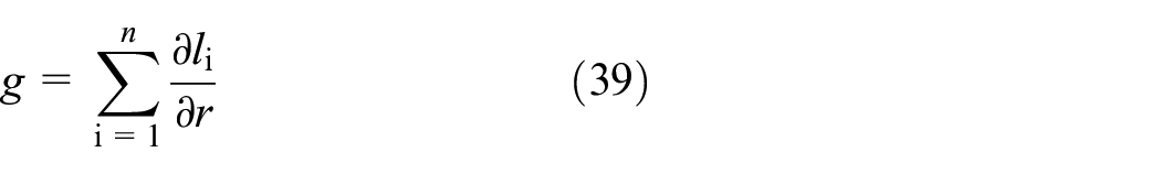
Because the linear and rotary movements in a single NC block would be completed simultaneously, we used the pseudo-distance instead of the linear distance to represent the total axial movements. Typically, the total pseudo-distance, ¹⁷ which will be called distance in the following, of the axial movements is determined as the root sum square of the movement in each axis, as shown in equation (7), in which $l$ is defined as the total pseudo-distance of the whole trajectory, and $l_i$ is defined as the distance on segment i of the trajectory. $(X_{i-1},Y_{i-1},Z_{i-1},A_{i-1},C_{i-1})$ and $(X_i,Y_i,Z_i,A_i,C_i)$ stand for the start and end positions of each axis in segment i defined in O_MXYZ, respectively.

$$l=\sum _{i=1}^n\sqrt{{(X_i-X_{i-1})}^2+{(Y_i-Y_{i-1})}^2+{(Z_i-Z_{i-1})}^2+{(A_i-A_{i-1})}^2+{(C_i-C_{i-1})}^2}=\sum _{i=1}^n{l}_i$$

(7)

To find the pseudo-distance, first, we derived the 4  4 homogeneous transformation matrix ${\mathbf{T}}_i$ and ${\mathbf{S}}_i$ with different kinematics of machine with the rotary angles $A$ and $C$ according to the steps in section 2.1. The general form of the transformation matrices can be represented as equations (8) and (9). We defined 3  3 matrices, ${{\mathbf{R}}_{\mathbf{T}}}_i$ and ${{\mathbf{R}}_{\mathbf{S}}}_i$ , as the rotary matrices, and 3  1 matrices, ${{\mathbf{L}}_{\mathbf{T}}}_i$ and ${{\mathbf{L}}_{\mathbf{S}}}_i$ , as the translation matrices in ${\mathbf{T}}_i$ and ${\mathbf{S}}_i$ , respectively. Then, the CL data in O_WXYZ can be transformed into the tool position in O_MXYZ with equation (10), defined as ${\mathbf{p}}_i$ . $(x_i,y_i,z_i)$ and $(X_i,Y_i,Z_i)$ represent the coordinates in O_WXYZ and O_MXYZ, respectively, in the toolpath segment i.

$${\mathbf{T}}_i=\left(\begin{array}{cc}{{\mathbf{R}}_{{\mathbf{T}}_i}}_{3\times 3}\hfill & {{\mathbf{L}}_{{\mathbf{T}}_i}}_{3\times 1}\hfill \\ \multicolumn{1}{c}{0_{1\times 3}}& 1\hfill \end{array}\right)$$

(8)

$${\mathbf{S}}_i=\left(\begin{array}{cc}{{\mathbf{R}}_{{\mathbf{S}}_i}}_{3\times 3}\hfill & {{\mathbf{L}}_{{\mathbf{S}}_i}}_{3\times 1}\hfill \\ \multicolumn{1}{c}{0_{1\times 3}}& 1\hfill \end{array}\right)$$

(9)

$${\mathbf{p}}_i=\left(\begin{array}{c}{X}_i\hfill \\ \multicolumn{1}{c}{Y_i}\\ \multicolumn{1}{c}{Z_i}\\ \multicolumn{1}{c}{1}\end{array}\right)={\mathbf{T}}_i·\left(\begin{array}{c}{x}_i\hfill \\ \multicolumn{1}{c}{y_i}\\ \multicolumn{1}{c}{z_i}\\ \multicolumn{1}{c}{1}\end{array}\right)-{\mathbf{S}}_i·\left(\begin{array}{c}0\hfill \\ \multicolumn{1}{c}{0}\\ \multicolumn{1}{c}{0}\\ \multicolumn{1}{c}{1}\end{array}\right)$$

(10)

We can define an offset vector $(p,q,r)$ as the movement from the original setup position. As shown in equation (11), the position of the start position of segment i can be transformed into the machine position with the offset of the setup position. Since the additional offset vector $(p,q,r)$ is a 3  1 vector, we need to add an element 0 to make it a homogeneous coordinate.

$$\begin{array}{c}\multicolumn{1}{c}{{\left({\mathbf{p}}_i\right)}_{\mathbf{offset}}={\mathbf{T}}_i·(\left(\begin{array}{c}{x}_i\hfill \\ \multicolumn{1}{c}{y_i}\\ \multicolumn{1}{c}{z_i}\\ \multicolumn{1}{c}{1}\end{array}\right)+\left(\begin{array}{c}p\hfill \\ \multicolumn{1}{c}{q}\\ \multicolumn{1}{c}{r}\\ \multicolumn{1}{c}{0}\end{array}\right))-{\mathbf{S}}_i·\left(\begin{array}{c}0\hfill \\ \multicolumn{1}{c}{0}\\ \multicolumn{1}{c}{0}\\ \multicolumn{1}{c}{1}\end{array}\right)}\\ ={\mathbf{p}}_i+\left(\begin{array}{cc}{{\mathbf{R}}_{{\mathbf{T}}_i}}_{3\times 3}\hfill & {{\mathbf{L}}_{{\mathbf{T}}_i}}_{3\times 1}\hfill \\ \multicolumn{1}{c}{0_{1\times 3}}& 1\hfill \end{array}\right)·\left(\begin{array}{c}p\hfill \\ \multicolumn{1}{c}{q}\\ \multicolumn{1}{c}{r}\\ \multicolumn{1}{c}{0}\end{array}\right)\hfill \end{array}$$

(11)

Because the fourth element of homogeneous coordinate is used for homogeneous transformation only, we can reduce the vector ${\left({\mathbf{p}}_{\mathbf{i}}\right)}_{\mathbf{offset}}$ from 4  1 to 3  1, as shown in equation (12). Then the start and end positions of segment i can be transformed to the machine positions with the consideration of the offset of the setup position, as shown in equations (12) and (13).

$${\left({\mathbf{p}}_i\right)}_{\mathbf{offset}}={\left(\begin{array}{c}{X}_i\hfill \\ \multicolumn{1}{c}{Y_i}\\ \multicolumn{1}{c}{Z_i}\end{array}\right)}_{\mathrm{offset}}={\mathbf{p}}_i+{\mathbf{R}}_{{\mathbf{T}}_i}·\left(\begin{array}{c}p\hfill \\ \multicolumn{1}{c}{q}\\ \multicolumn{1}{c}{r}\end{array}\right)$$

(12)

$${\left({\mathbf{p}}_{i-1}\right)}_{\mathbf{offset}}={\left(\begin{array}{c}{X}_{i-1}\hfill \\ \multicolumn{1}{c}{Y_{i-1}}\\ \multicolumn{1}{c}{Z_{i-1}}\end{array}\right)}_{\mathrm{offset}}={\mathbf{p}}_{i-1}+{\mathbf{R}}_{{\mathbf{T}}_{i-1}}·\left(\begin{array}{c}p\hfill \\ \multicolumn{1}{c}{q}\\ \multicolumn{1}{c}{r}\end{array}\right)$$

(13)

Here we defined $\mathrm{\Delta }{X}_i,\mathrm{\Delta }{Y}_i,\mathrm{and}\mathrm{\Delta }{Z}_i$ as the following equation by subtracting equation (13) from equation (12),

$$\begin{array}{c}\multicolumn{1}{c}{{\left(\begin{array}{c}\mathrm{\Delta }{X}_i\hfill \\ \multicolumn{1}{c}{\mathrm{\Delta }{Y}_i}\\ \multicolumn{1}{c}{\mathrm{\Delta }{Z}_i}\end{array}\right)}_{\mathrm{offset}}={\left(\begin{array}{c}{X}_i\hfill \\ \multicolumn{1}{c}{Y_i}\\ \multicolumn{1}{c}{Z_i}\end{array}\right)}_{\mathrm{offset}}-{\left(\begin{array}{c}{X}_{i-1}\hfill \\ \multicolumn{1}{c}{Y_{i-1}}\\ \multicolumn{1}{c}{Z_{i-1}}\end{array}\right)}_{\mathrm{offset}}}\\ =({\mathbf{p}}_i-{\mathbf{p}}_{i-1})+({\mathbf{R}}_{{\mathbf{T}}_i}-{\mathbf{R}}_{{\mathbf{T}}_{i-1}})·\left(\begin{array}{c}p\hfill \\ \multicolumn{1}{c}{q}\\ \multicolumn{1}{c}{r}\end{array}\right)\hfill \end{array}$$

(14)

In addition, we defined $\mathrm{\Delta }{A}_i\mathrm{and}\mathrm{\Delta }{C}_i$ as the movements of two rotary axes in segment i, as shown in equations (15) and (16). Thus, the pseudo-distance of segment i, l_i, can be calculated by using equation (17), with the consideration of the offset of the setup position.

$$\mathrm{\Delta }{A}_i=A_i-A_{i-1}$$

(15)

$$\mathrm{\Delta }{C}_i=C_i-C_{i-1}$$

(16)

$$l_i=\sqrt{\mathrm{\Delta }{X_i}^2+\mathrm{\Delta }{Y_i}^2+\mathrm{\Delta }{Z_i}^2+\mathrm{\Delta }{A_i}^2+\mathrm{\Delta }{C_i}^2}$$

(17)

As shown in equation (17), it is well-known that the Euclidean distance is a convex function. ¹⁸ In other words, the equation is a typical convex function, we called the distance function $f$ . However, the domain of the distance function $f$ , F, is different from the machinable domain which exists the offset vector $(p,q,r)$ , which is denoted by G. Thus, the mapping from F to G is needed.

Since the rotary movements stay the same within the transformation from O_WXYZ to O_MXYZ, the terms $\mathrm{\Delta }{A}_i$ and $\mathrm{\Delta }{C}_i$ are constant. Therefore, the terms would not affect the convexity of the distance function. Thus, we can simplify the equation by eliminating the terms $\mathrm{\Delta }{A}_i$ and $\mathrm{\Delta }{C}_i$ from equation (17). The simplied vector is denoted by ${\mathbf{L}}_{\mathbf{i}}$ ,

$${\mathbf{L}}_{\mathbf{i}}=(\mathrm{\Delta }{X}_i,\mathrm{\Delta }{Y}_i,\mathrm{\Delta }{Z}_i)$$

(18)

Then we can redefine the distance function of segment i, ${l_i}^{*}$ , which is the Euclidean norm of ${\mathbf{L}}_{\mathbf{i}}$ ,

$${l_i}^{*}=\sqrt{\mathrm{\Delta }{X_i}^2+\mathrm{\Delta }{Y_i}^2+\mathrm{\Delta }{Z_i}^2}=\Vert {\mathbf{L}}_{\mathbf{i}}\Vert =f({\mathbf{L}}_{\mathbf{i}})$$

(19)

The vector ${\mathbf{L}}_{\mathbf{i}}$ can be represented as equation (20) from equation (14) with an affine mapping,

$$\begin{array}{c}\multicolumn{1}{c}{{\mathbf{L}}_{\mathbf{i}}=\left(\begin{array}{c}\mathrm{\Delta }{X}_i\hfill \\ \multicolumn{1}{c}{\mathrm{\Delta }{Y}_i}\\ \multicolumn{1}{c}{\mathrm{\Delta }{Z}_i}\end{array}\right)=({\mathbf{R}}_{{\mathbf{T}}_{\mathbf{i}}}-{\mathbf{R}}_{{\mathbf{T}}_{\mathbf{i}-1}})·\left(\begin{array}{c}p\hfill \\ \multicolumn{1}{c}{q}\\ \multicolumn{1}{c}{r}\end{array}\right)}\\ +({\mathbf{p}}_{\mathbf{i}}-{\mathbf{p}}_{\mathbf{i}-1})=\mathbf{M}·{\mathbf{d}}_{\mathbf{w}}+\mathbf{N}\hfill \end{array}$$

(20)

where ${\mathbf{R}}_{{\mathbf{T}}_{\mathbf{i}-1}}$ and ${\mathbf{R}}_{{\mathbf{T}}_{\mathbf{i}}}$ are the rotary matrices in the transformation relative to the start position ${\mathbf{p}}_{\mathbf{i}-1}$ and the end position ${\mathbf{p}}_{\mathbf{i}}$ , respectively. $\mathbf{M}$ is the matrix obtained by subtracting ${\mathbf{R}}_{{\mathbf{T}}_{\mathbf{i}-1}}$ from ${\mathbf{R}}_{{\mathbf{T}}_{\mathbf{i}}}$ , which is a linear transformation in the machinable domain G. The vector ${\mathbf{d}}_{\mathbf{w}}$ is the offset vector $(p,q,r)$ in G. $\mathbf{N}$ is a vector in the domain F.

The distance function now is $f:{\mathbf{R}}^3\to \mathbf{R}$ , $\mathbf{M}\in {\mathbf{R}}^{3\times 3}$ , and $\mathbf{N}\in {\mathbf{R}}^3$ , then we can define the function $g:{\mathbf{R}}^3\to \mathbf{R}$ by

$$g({\mathbf{d}}_{\mathbf{w}})=f(\mathbf{M}·{\mathbf{d}}_{\mathbf{w}}+\mathbf{N})=f({\mathbf{L}}_{\mathbf{i}})$$

(21)

which maps the distance function $f$ from the domain F to the domain G. We can define $u,v\in {\mathbf{R}}^3$ in the domain of the function $g$ . Then $\forall \lambda \in [0,1]$ ,

$$\begin{array}{c}\multicolumn{1}{c}{g(\lambda u+(1-\lambda )v)=f(\mathbf{M}(\lambda u+(1-\lambda )v)+\mathbf{N})}\\ =f(\lambda (\mathbf{M}u+\mathbf{N})+(1-\lambda )(\mathbf{M}v+\mathbf{N}))\hfill \\ \le f(\lambda (\mathbf{M}u+\mathbf{N}))+f((1-\lambda )(\mathbf{M}v+\mathbf{N}))\hfill \\ =\lambda f(\mathbf{M}u+\mathbf{N})+(1-\lambda )f(\mathbf{M}v+\mathbf{N})\hfill \\ =\lambda g(u)+(1-\lambda )g(v)\hfill \end{array}$$

(22)

The equation shows that the function $g$ is a convex function as well. Then, the objective function, which is the total distance $l^{*}$ , can be represented as

$$l^{*}=\sum _{i=1}^n{l_i}^{*}=\sum _{i=1}^{n}g({\mathbf{d}}_{\mathbf{w}})$$

(23)

The objective function, $l^{*}$ , is a non-negative weighted sum of convex functions. We can define non-negative weights $\alpha ,\beta \ge 0$ and $g_1,g_2$ as convex function. Follow the definition of a convex function, $\forall \lambda \in [0,1]$ ,

$$g_1(\lambda u+(1-\lambda )v)\le \lambda g_1(u)+(1-\lambda ){\mathrm{g}}_1(v)$$

(24)

$$g_2(\lambda u+(1-\lambda )v)\le \lambda g_2(u)+(1-\lambda ){\mathrm{g}}_2(v)$$

(25)

Then, $\forall \lambda \in [0,1]$ ,

$$\begin{array}{c}h(\lambda u+(1-\lambda )v)=\alpha ·g_1(\lambda u+(1-\lambda )v)\hfill \\ +\beta ·g_2(\lambda u+(1-\lambda )v)\hfill \\ \le \alpha ·(\lambda g_1(u)+(1-\lambda ){\mathrm{g}}_1(v))+\beta ·(\lambda g_2(u)\hfill \\ +(1-\lambda ){\mathrm{g}}_2(v))=\lambda h(u)+(1-\lambda )\mathrm{h}(v)\hfill \end{array}$$

(26)

where $h=\alpha ·g_1+\beta ·g_2$ , which can be proved as a convex function. With the proof above, the objective function, $l^{*}$ , is a convex function in machinable domain G. In other words, there exists a global minimum that is the same as the local minimum in the set of ${l_n}^{*}$ with a spatial set of setup offset variables ${\mathbf{d}}_{\mathbf{w}}$ . The objective of the optimization problem is to determine the optimal setup position of the workpiece to minimize the total distance for the axial movements in the machinable domain,

$$\begin{array}{c}\underset{{\mathbf{d}}_{\mathbf{w}}}{\mathrm{minimize}}{l}^{*}=\sum _{i=1}^n{l_i}^{*}=\sum _{i=1}^{n}g({\mathbf{d}}_{\mathbf{w}})\hfill \\ \mathrm{subject}\mathrm{to}\mathrm{the}\mathrm{offset}\mathrm{vector}{\mathbf{d}}_{\mathbf{w}}\mathrm{in}\mathrm{the}\mathrm{machinable}\mathrm{domain}\mathbf{G}\hfill \end{array}$$

(27)

Next, we proposed an algorithm to search the optimal result within the constraint region of the machinable domain. ¹⁹

Method to determine the optimal setup position

The objective function has been proven as a convex function, which means that the local minimum is the same as the global minimum in a dexel. Hence, we can use the gradient descent method to search for the minimum in the machinable domain for each dexel. ²⁰ The machinable domain is the collection of all possible setup position without having problems including over travel limits of any linear axis and collision between the tool assembly and the machine components. However, the machinable domain is too complicated so that practically it can be described in discretized dexel, which is pixels on the XY plane with depth information in the Z-axis, as shown in Figure 5.

Figure 5.

Represent domain with discretized dexels. Each dexel has one local minimum (blue layer), then compare and select the minimal value as a global minimum in the domain (red layer).

To ensure that the global minimum is selected within the machinable domain, we need to check each local minimum to obtain the global minimum. The local minimum is the minimum in each dexel. Nevertheless, there might exist certain minimal values that are the same as the global minimum. Thus, we proposed another criterion to select the global minimum from the same minimum values at different positions. The criterion is to choose the position closest to the center of the worktable in order to meet the common setting in industry. Eventually, the optimal workpiece setup position with the shortest distance of the axial movements can be obtained.

As a result of optimization, $d_{\mathrm{opt}}$ refers to the shortest total axial movements with the workpiece in the optimal setup position. $d_{\mathrm{org}}$ refers to the original distance of the workpiece in the original setup position. In general, the original setup position is set at the center of the pallet table. To compare $d_{\mathrm{opt}}$ with $d_{\mathrm{org}}$ , $d_R$ is defined in equation (28) as a percentage of reduced axial movements. Moreover, the optimized and original machining time $t_{\mathrm{opt}}$ and $t_{\mathrm{org}}$ are recorded in the case study. $t_R$ is defined as the percentage of the reduced machining time, as shown in equation (29).

$$d_R=\frac{d_{\mathrm{org}}-d_{\mathrm{opt}}}{d_{\mathrm{org}}}\times 100\mathrm{\%}$$

(28)

$$t_R=\frac{t_{\mathrm{org}}-t_{\mathrm{opt}}}{t_{\mathrm{org}}}\times 100\mathrm{\%}$$

(29)

Experimental environment and setup

Experimental environment

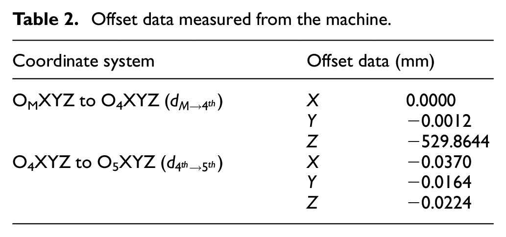
In this research, the toolpaths would be planned in NX software (Siemens, Germany) and then simulated on a TATC machine (Model Number UX300, Quaser, Taiwan), as shown in Figure 6(a), which is equipped with a Heidenhain iTNC530 controller. The specifications of the machine, including the travel limit (Table 1) and the offset data of the coordinate system (Table 2), were applied to calculate the optimal workpiece setup position. The offset data from O₅XYZ to O_wXYZ was set to zero because we coincided these two points with the setup setting on machine. The dimensions of the five-axis machine ${\mathbf{d}}_{\mathrm{M}\to 4^{\mathrm{th}}}$ and ${\mathbf{d}}_{4^{\mathrm{th}}\to 5^{\mathrm{th}}}$ were measured by using the Heidenhain probe TS740 and the Heidenhain calibration sphere KKH100 with the CYCLE451 command built in the Heidenhain controller, as shown in Figure 6(b). After that, we machined the parts to obtain the cutting time for comparison among different workpiece setup positions.

Figure 6.

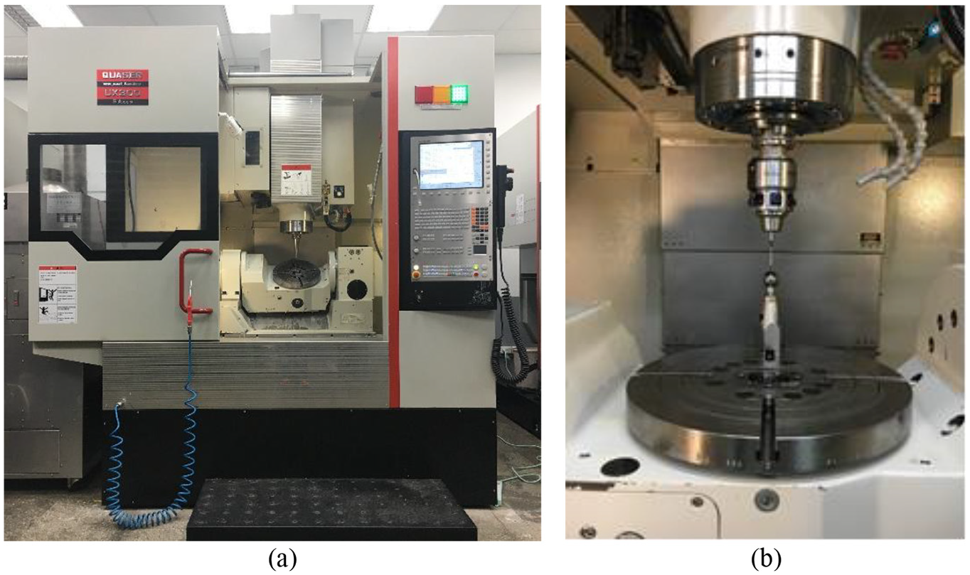
(a) Quaser UX300 five-axis machine with a Heidenhain controller. (b) Measuring the machine kinematics by a Heidenhain probe TS740 and a calibration sphere KKH100.

Table 1.

Quaser UX300 axis limits.

Machine travel	Negative limit	Positive limit
X	−205 mm	205 mm
Y	−305 mm	305 mm
Z	−500 mm	0 mm
A	−120°	30°
C	360° continuous

Table 2.

Offset data measured from the machine.

Coordinate system	Offset data (mm)
OMXYZ to O4XYZ ( $d_{M\to 4^{\mathrm{th}}}$ )	X	0.0000
	Y	−0.0012
	Z	−529.8644
O4XYZ to O5XYZ ( $d_{4^{\mathrm{th}}\to 5^{\mathrm{th}}}$ )	X	−0.0370
	Y	−0.0164
	Z	−0.0224

Example of optimization program process

In this section, we would use a simple example to demonstrate the process of optimization. The example is a linear cutting toolpath. The CL data are shown as follows,

• FEDRAT/MMPM, 1000.0000

• GOTO/0.000, 0.000, 0.000, 0.000, 0.000

• GOTO/10.000, 20.000, 30.000, –40.000, 50.000

The start position $(x_1,y_1,z_1,A_1,C_1)$ is $(0,0,0,0°,0°)$ , and the end position $(x_2,y_2,z_2,A_2,C_2)$ is $(10,20,30,-40°,50°)$ defined in O_WXYZ. The unit of the linear axes X, Y, and Z was millimeter, and that of the rotary axes A and C was degree. The length of the cutting toolpath $d_{\mathrm{cut}}$ was 37.4166 mm, which was calculated as a root sum square distance from $(0,0,0)$ to $(10,20,30)$ ,

$$d_{\mathrm{cut}}=\sqrt{{(x_2-x_1)}^2+{(y_2-y_1)}^2+{(z_2-z_1)}^2}=37.4166$$

(30)

The first step was to divide the toolpath into small segments with the interpolation time of the controller $t_{\mathrm{ipt}}$ , which was 0.1 ms for the iTNC530 controller. Because the feed rate F in the CL data was 1000 mm/min, the interpolation distance $d_{\mathrm{ipt}}$ was calculated as follow,

$$d_{\mathrm{ipt}}=F·t_{\mathrm{ipt}}/60000=0.0017$$

(31)

Then we can extract the first segment of the cutting path by using $r_{\mathrm{ipt}}$ , the ratio of the interpolation distance $d_{\mathrm{ipt}}$ and the length of the cutting toolpath $d_{\mathrm{cut}}$ . In this example,

$$r_{\mathrm{ipt}}=d_{\mathrm{ipt}}/d_{\mathrm{cut}}=0.0017/37.4166=4.5434\times {10}^{-5}.$$

(32)

With the interpolation ratio $r_{\mathrm{ipt}}$ , the interpolated lengths or angles can be calculated as $(0.4543,0.9087,1.3630,-1.8174°,2.2717°)\times 10^{-3}$ between the start position and the end position along the five axes of the machine tool.

Next, we focused on the interpolation segment between position A $(0,0,0,0°,0°)$ and position B $(0.4543,0.9087,1.3630,-1.8174°,2.2717°)\times 10^{-3}$ . The transformation matrices related to both positions can be calculated as follows by using equations (1) and (2). Here we substitute coordinate of position A and B, the kinematics data in Table 2 into the transformation matrices, and the cutting tool we used is 100.125 mm measured from the spindle nose to the tooltip along the –Z direction.

$${\mathbf{T}}_{\mathbf{A}}=\left(\begin{array}{cccc}1\hfill & 0\hfill & 0\hfill & -0.0370\hfill \\ \multicolumn{1}{c}{0}& 1\hfill & 0\hfill & -0.0176\hfill \\ \multicolumn{1}{c}{0}& 0\hfill & 1\hfill & -529.8868\hfill \\ \multicolumn{1}{c}{0}& 0\hfill & 0\hfill & 1\hfill \end{array}\right)$$

(33)

$${\mathbf{S}}_{\mathbf{A}}=\left(\begin{array}{cccc}1\hfill & 0\hfill & 0\hfill & 0\hfill \\ \multicolumn{1}{c}{0}& 1\hfill & 0\hfill & 0\hfill \\ \multicolumn{1}{c}{0}& 0\hfill & 1\hfill & -100.125\hfill \\ \multicolumn{1}{c}{0}& 0\hfill & 0\hfill & 1\hfill \end{array}\right)$$

(34)

$${\mathbf{T}}_{\mathbf{B}}=\left(\begin{array}{cccc}1\hfill & 3.9649\times {10}^{-5}\hfill & 0\hfill & -0.0370\hfill \\ \multicolumn{1}{c}{-3.9649\times {10}^{-5}}& 1\hfill & -3.1720\times {10}^{-5}\hfill & -0.0176\hfill \\ \multicolumn{1}{c}{-1.2576\times {10}^{-9}}& 3.1720\times {10}^{-5}\hfill & 1\hfill & -529.8868\hfill \\ \multicolumn{1}{c}{0}& 0\hfill & 0\hfill & 1\hfill \end{array}\right)$$

(35)

$${\mathbf{S}}_{\mathbf{B}}=\left(\begin{array}{cccc}1\hfill & 0\hfill & 0\hfill & 0\hfill \\ \multicolumn{1}{c}{0}& 1\hfill & 0\hfill & 0\hfill \\ \multicolumn{1}{c}{0}& 0\hfill & 1\hfill & -100.125\hfill \\ \multicolumn{1}{c}{0}& 0\hfill & 0\hfill & 1\hfill \end{array}\right)$$

(36)

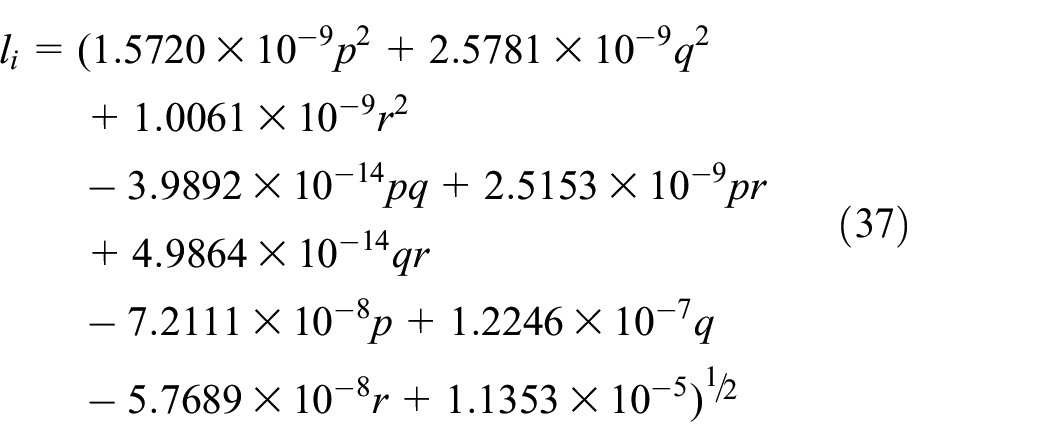
With the elements in the transformation matrices, we can use equation (17) to obtain the distance function of segment one as

$$\begin{array}{l}{l}_i=(1.5720\times {10}^{-9}{p}^2+2.5781\times {10}^{-9}{q}^2\\ +1.0061\times {10}^{-9}{r}^2\\ -3.9892\times {10}^{-14}pq+2.5153\times {10}^{-9}pr\\ +4.9864\times {10}^{-14}qr\\ -7.2111\times {10}^{-8}p+1.2246\times {10}^{-7}q\\ -5.7689\times {10}^{-8}r+1.1353\times {10}^{-5}{)}^{1/2}\end{array}$$

(37)

Then we can derive the gradient of the distance function of segment one as the partial derivative of the distance function with respect to $r$ , which is the offset of the workpiece setup position along the Z-axis, as shown in equation (38). After adding all of the gradients, we can obtain the total gradient as equation (39).

$$\frac{\partial l_i}{\partial r}=\frac{(1.0061\times {10}^{-9}r+2.5153\times {10}^{-9}p+4.9864\times {10}^{-14}q-5.7689\times {10}^{-8})}{2l_i}$$

(38)

$$g=\sum _{\mathrm{i}=1}^n\frac{\partial l_{\mathrm{i}}}{\partial r}$$

(39)

With the numerical gradient $g$ , we can calculate the optimal value $r$ by using the gradient descent method in each dexel. For instance the dexel at x and y position $(0,0)$ , the gradient is calculated by substitute $p$ = $q$ = 0 into equation (39). The range of $r$ at the $(0,0)$ position was [4,425] along the Z-axis, which was obtained from the machinable domain as shown in Figure 7(a). The machinable domain is calculated by the algorithm we proposed. ¹⁹ Thus, the local minimum value can be obtained at 4 mm offset along the Z-axis on the dexel at $(0,0)$ position, as shown in Figure 7(b), where the relationship between the machining distance and the offset value is illustrated. After the optimization program computed the minimum for each dexel, the global minimum value was found at $(10,-35)$ with the optimal offset value 4 mm along the Z-axis, which is the position of the minimum value shown in the contour plot of Figure 7(c).

Figure 7.

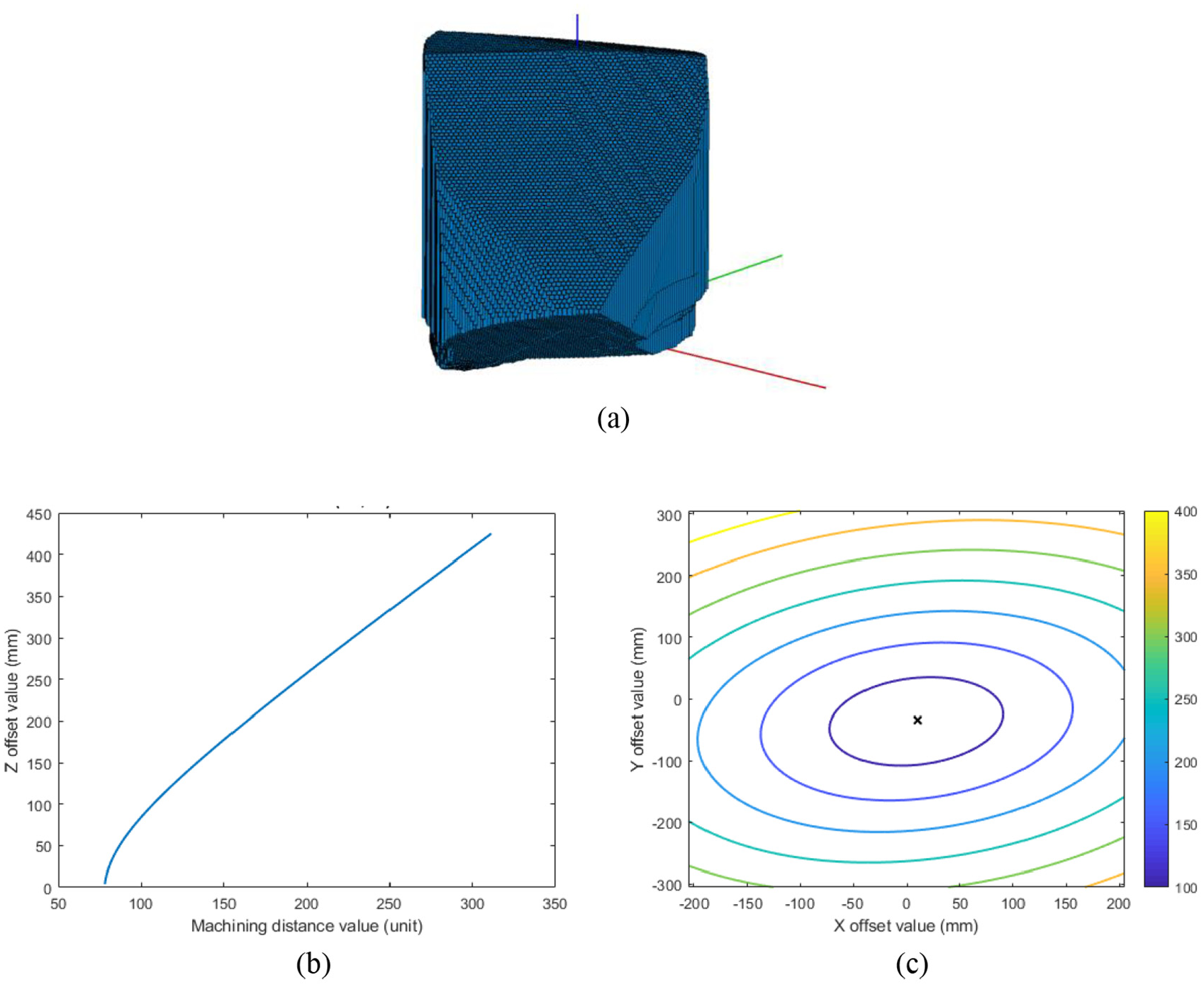
(a) Workpiece machinable domain results of the linear toolpath in the example. (b) Machining distance value versus Z offset value at position X = 0 and Y = 0. (c) Contour plots of axial movements on the XY plane at Z = 4. “x” shows the optimal setup offset.

Case study

A cuboid with a curved channel was used to demonstrate our study, as shown in Figure 8(a). The channel is altered from 30 mm to 28 mm in diameter along a spline curve. It can be machined from both sides at one-time setup on a five-axis machine tool. The origin of the workpiece was at the center of the bottom surface, which is coincided with the center of the worktable, as shown in Figure 8(b). The toolpath was planned to finish the channel from both sides with a 80 mm long, 10 mm in diameter ball-milling tool. The total length of the tool assembly is 230 mm, as shown in Figure 9.

Figure 8.

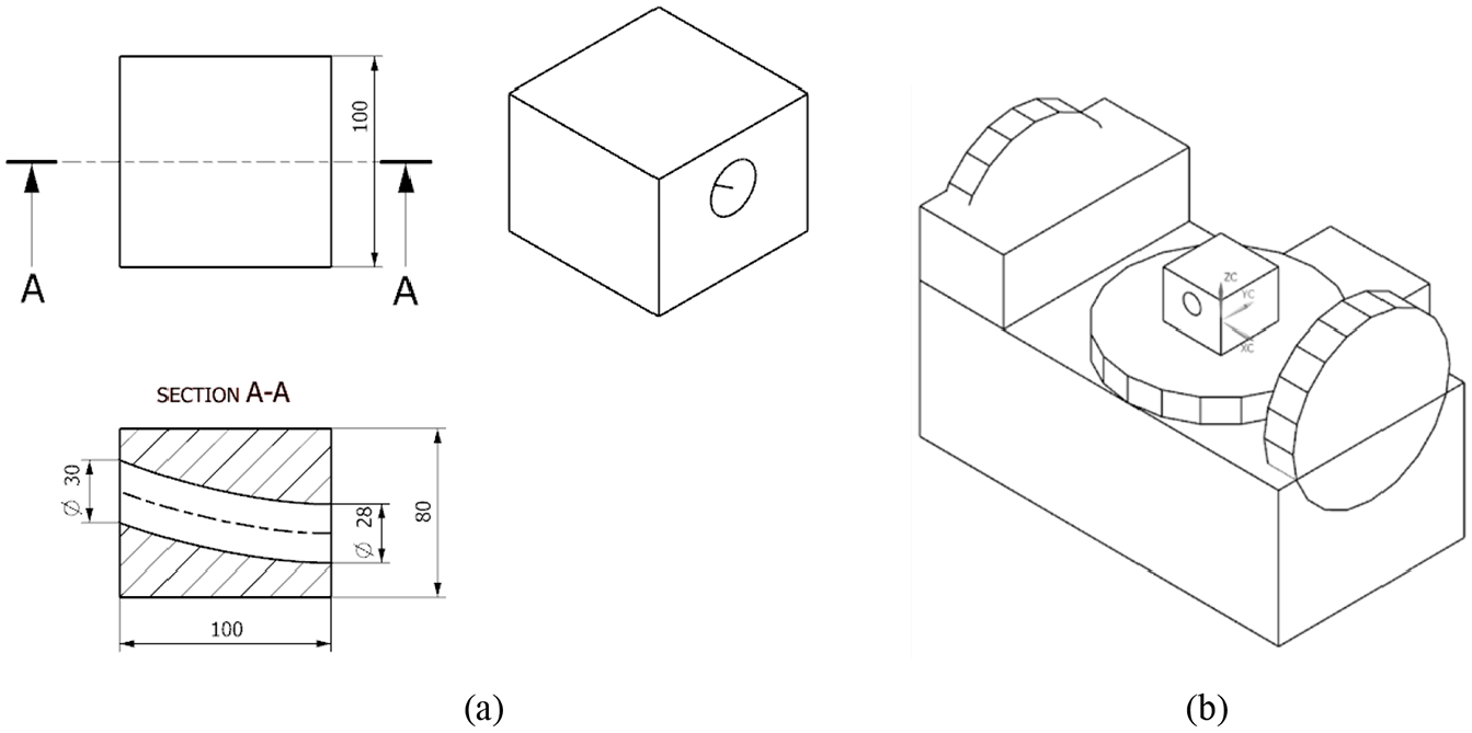
(a) Channel from 30 mm to 28 mm in diameter along a spline curve. (b) Initial workpiece setup on machine.

Figure 9.

Toolpath for the channel: (a) left-side; (b) right-side.

According to the workpiece’s machinable domain, it was found that the workpiece must be raised 123 mm along the Z-axis from the orginial workpiece setup position, so that the workpiece is machinable. Figure 10 shows a contour plot of the total axial movements distance. The figure shows that the original setup position, the black “o” at (0, 0, 0), is not machinable. Within the constraint of the machinable domain, the modified setup position, the blue “o” at (0, 0, 123), gives the distance of 64653 units. However, we can find an optimal setup position, the orange “o” at (0, 90, 65), to reduce the distance. The global minimum of optimal setup position at (0, 90, 65) gives the shortest distance of 53,816 units.

Figure 10.

Contour plot of axial movements results on the section (a) YZ plane at X0, and (b) XY plane at Z65. The boundaries of the cross section of the machinable domain are the black lines. The black “o” refers to the origin setup position, the blue “o” refers to the modified setup position and the orange “o” refers to the optimal setup position.

Three parts with three different setup positions listed in Table 3 were machined, as illustrated in Figure 11. Because the part put at (0, 0, 0) is not machinable, we move the part to the modified setup position (0, 0, 123) to make it machinable, and the total axial movements was calculated as 64,653 units as listed in Table 3. The real machining time was 561 s. Then we set the part at the optimal setup position, and the total axial movements was calculated as 53,816 units, which was 16.76% less than the those for the part put at the modified setup position. The machining time was 501 s, which was 10.70% less than that for the part put at the modified setup position. Because the total axial movements were very complicated, the reduction in distance was not very consistent with that in machining time. Based on the results, it is demonstrated that the algorithm proposed can find the optimum setup position to reduce the machining time effectively.

Table 3.

Calculated and real machining results of the channel.

Workpiece setup position	Distance	Reduced distance	Machining time	Reduced time	Machinable
Origin (X0, Y0, Z0)	42,169	−	−	−	No
Modified result (X0, Y0, Z123)	64,653	−	561 s	−	Yes
Optimal result (X0, Y90, Z65)	53,816	16.76%	501 s	10.70%	Yes

Figure 11.

(a) The real cutting process and (b) the section view of the channel.

Conclusion

In this paper, we derived the kinematics for each type of five-axis machine tools. Then, we used the general transformation matrix to derive the optimization equation and the gradient descent method to find the global minimum. A case is presented to verify the proposed method and the total axial movements were reduced by 16.76%, and the machining time was reduced by 10.70% if we set up the workpiece at the optimal position. The proposed method can substantially reduce the machining time for the five-axis machining, which is practically important to the machining industry.