Sage Journals: Discover world-class research

Abstract

The initial design of baggage-lifting machine structures is primarily based on safety and reliability, but they are often damaged because of unforeseen circumstances and overloads. In this study, a machine learning–based logistic regression method for detecting structural damage to bolted truss structures during field work is proposed. Multiple strain gauges attached to the front of the truss model record the amount of deformation occurring in the member when the vertical load generated at the end of the model is applied. In this process, the scatter or error caused by the sample is analyzed, and the data processing method is presented. Experimental results demonstrate that this method provides a good quantitative basis for fault detection, and it can be effectively applied to partial representative data when handling large datasets.

Keywords

Failure detection fatigue load truss structure machine learning PHM

Introduction

Fault analysis and reliability analysis are essential to ensure the long-term usability of devices, and an analysis of environmental factors, including structural analysis and material selection, may also be helpful. Methods for obtaining the characteristic values of a structure can be classified into dynamic and static identification methods. Among them^1,2 the static identification method requires only structural stiffness, and several studies have been published using strain gauges as a method for obtaining data in this process; artificial damage was made to the joints or bulk material connected to the bridge or reduced by lab-scale model, after which strain gauges and strain transducers were attached to measure strain during loading. In the subsequent data processing, damage detection was calculated by efficiently using neural networks,^3,4 and the physical analysis was compared.^4–6 In order to overcome the limitations of data-driven models, it is also possible to create a hybrid model with the physical model to increase accuracy and compare the degree of improvement in reliability with that of the individual models.^7–9

By presenting a method of identifying structural parameters using element strain measurement for numerical examples including two-dimensional truss and frame structure, strain measurement is more accurate than displacement measurement that does not require a reference frame and it is easier to measure large structures such as bridges and buildings. Also, the damage prediction study based on the acceleration signal measurement proved its reliability by applying it to Howe and Bailey trusses after subsequent statistical processing. As the research on the static approach of structural state monitoring was conducted, it progressed to the stage where it is possible to accurately identify the damage location of the structure even in the data including noise.^10–13

The previously described steps are from the process of SHM to the stage of operational evaluation-data acquisition-feature extraction, and the last step is assessment of the damage condition, which can be called pattern recognition of machine learning. As a research applying machine learning, the steel pipe with piezoelectric wafers was studied on the damage detection placed mass scatters at multiple locations and various environmental conditions for experimentally verifying the effectiveness and robustness of data-driven framework of SHM. The detected data characterized 365 features extracted by signal processing techniques, and five machine learning classifiers showed a high accuracy close to 100% in a randomized test. Among several classifier algorithms that can be used in machine learning, RFC random forest classifier, KNN, and support vector machine algorithms were applied to the same damage/non-damage conditions to compare the prediction rate.^14–16

In this study, the strain signal generated when the cyclic fatigue load is applied to the truss model assembled in a vertically symmetrical form is extracted through the strain gauge. The extracted signal is then compared with that generated when the same load is applied to the model after replacement with section steel containing artificial cracks. The data-driven model is classified into normal and fault data using the logistic regression-classification machine learning technique. A method and a data processing approach for the method are proposed to identify a failure when selecting a random strain channel. In addition, the process is demonstrated to be able to identify failure in the same manner even when only partial data is used.

Fault decision methodology with logistic regression

In this paper, the logistic regression method was used to determine whether the structure is faulty, and the steps are performed in the order shown in the block diagram of Figure 1.

Figure 1.

Block diagram of learning process.

First, the data was cleansing and normalizing for a total of 48 data consisting of 24 normal data and 24 failure data. In this process, the initial and last data are deleted, such as when loading and unloading. Logistic regression defines the normal value of 0 and the failure value of 1 for time series data, and starts the process of 24 channels.

The second process is data selection. At this time, one of 24 normal data and one of 24 failure data were randomly selected and used for logistic regression. In this paper, a total of 552 machine learnings was performed in one experiment to calculate error rates. Octave was used in machine learning.

The third process is to confirm the error rate and determine whether the selected failure data contains a crack. A decision boundary layer between two selected data on logistic regression was generated, and the error rate can be calculated by using this layer as a reference and how to distinguish normal-fault data accurately.

The final process is failure determination. A total of 552 learnings, which can be done in one experiment, is executed first, and the error rate when there is failure data including cracks and the error rate when it does not are calculated respectively. And the final average was calculated. The coefficients a and b of the first linear equation (y = ax+b), decision boundary layer are calculated from the results of machine learning using gradient decent. The decision boundary layer is drawn based on the calculated formula, and if the error rate is 70% or more at this time, it is determined that the decision boundary layer correctly distinguishes normal data from fault data.

θ_{j} ≊ θ_{j} - α \frac{\partial}{\partial θ_{j}} J (θ_{0}, θ_{1})

(1)

J (θ_{0}, θ_{1}) = \frac{1}{2 m} \sum_{i = 1}^{m} {(h_{θ} (x^{(i)}) - y^{(i)})}^{2}

(2)

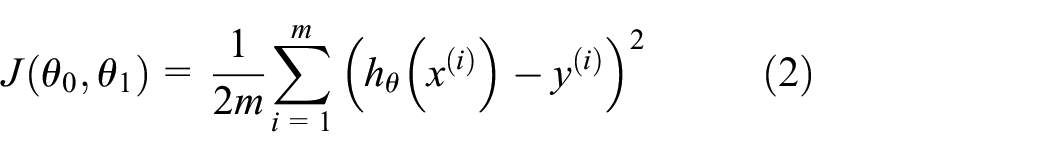
Equation (1) is for intuitively explaining the gradient decent algorithm, and machine learning has pounded the optimal decision boundary layer by repeating the calculation. The alpha value is the learning rate and is used as a constant that determines the change of the i+ 1st slope, and it simultaneously update j = 0 and j = 1. Equation (2) is an equation for calculating the cost function J used in equation (1), minimizing the sum of the square of the difference between the actual data value y value and the assumed linear equation h up to the total number of training samples m, that is, minimizing J. That is the purpose of machine learning.

Additionally, an exceptional case was explained where cracks were included even in an error rate of 70% or more. And preprocessing of partial data was described for using logistic regression and compared with the entire data as plotting in a graph.

Experiment

The target model was devised from the tower crane used to lift objects at the construction site. The tower crane, which is designed in the form of a truss, is bent at a fixed point when lifting a heavy object. In the experiment, in order to approximate the behavior of an actual tower crane, the same truss structure was assembled in a symmetrical shape and a load was applied in the uniaxial direction. As shown in Figure 2, when a load is applied to the truss structure, a bending load occurs at the assembled end.

Figure 2.

Attached strain gauge location and spots of replaced steel angle in the truss model as (a) front view and (b) rear view.

A total of 24 strain gauges for strain measurement were attached symmetrically to the front and rear of the truss model in Figure 2. A small truss model was manufactured for mounting on the tester, and a small beams and channels were used for fastening with bolts. The bolt was tightened using M6 and M8 size high-strength bolts, and the torque wrench was tightened to each bolt with a constant torque.

The section steel used in the experiment is shaped as defined in the Korea standard, and the material is SS400.^17,18 Two types of section steel are used. First one, the equilateral L-type has the same cross section length of 30 × 30 mm and the thickness of 3 mm. The second is a lipped channel with a cross section of 60 × 30 × 10 mm and a thickness of 3.2 mm. It is a vertically symmetrical model which generates repulsive force at the fixed end as a supporter when it is loaded at the front. It simulates the result of the actual crane model lifting the baggage, implementing the same shape, and the top and bottom of the jig part of the tester used are symmetrical because of the constraint that is in the same line. The block used for the fixed end and the plate part bites by the machine to load the truss at the front part were used as S45C. A universal testing machine with a 250 kN load capacity (Quasar 250, Galdabini, Italy) was used for loading, and the strain value was acquired by a data logger via the strain gauges. Figure 3 shows the truss model mounted on the tester.

Figure 3.

Truss model assembled with steel angles and conditions.

The tensile loads were statically loaded on the truss structures, and the experimental conditions were determined based on the resulting stress-strain curve. The displacement values corresponding to the load conditions within the elastic range were repeated at regular intervals throughout the experiment on the normal structure. After that, the structure was separated from the test machine, and the deformation signal was replaced to include a crack with a width of 1 mm and depth of 20 mm, formed by artificial processing, in the center of the section steel. The strain signal in the structure without the crack was compared with that in the structure with the crack. Through this experiment, it is possible to compare the signal measured in the normal structure (before the replacement with the cracked section steel) with that measured in the structure after the replacement. However, as can be seen from the conditions, the amount of displacement and frequency applied to the structure are not large enough to accumulate damage. Therefore, in this experiment, it is important to confirm the immediate change of the strain gauge depending on whether including the failure or not. There are four locations for the replacement with the cracked section steel, and Table 1 shows the displacement range, frequency, and location for each damage scenario.

Table 1.

Test conditions.

Damage scenario	Trial	Crack location	Test range (mm)	Frequency (Hz)
#1	1	F-6	1.5–2.5	0.2
#1	2	F-6
#2	1	F-11
#2	2	F-11
#3	1	R-11
#3	2	R-11
#4	1	R-6
#4	2	R-6

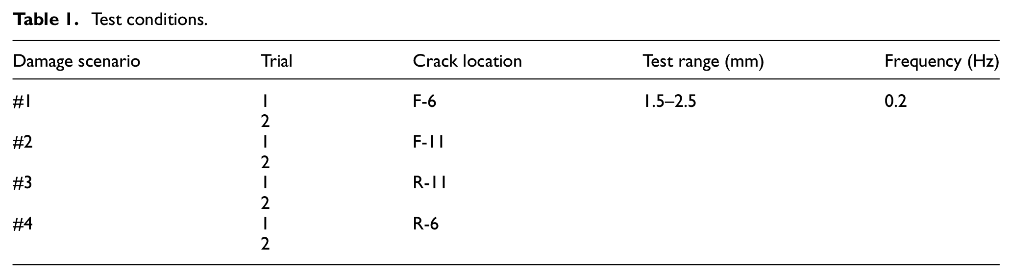
Figure 4(a) shows the strain value at the strain gauge channel CH 15, which is attached to the cracked section steel which replaced the shape of R-6 in the damage scenario #4, resulting in the strain phase between the normal structure and the fault structure turning 180 degrees. It was found that 4(b), (c) is the strain value at CH 13 and CH 18, which are strain gauge channels attached near the cracked steel. Moreover, the absolute value of the maximal strain on the fault structure is higher than that on the normal structure, and the absolute value of the minimum strain on the fault structure is lower than that on the normal structure. Thus, it can be seen that the measured strain signals differ based on whether or not the structure contains cracks.

Figure 4.

Strain signal comparison on different strain gauge channels on (a) CH 15 (on cracked member), (b) CH 13 (on non-cracked member), and (c) CH 18 (on non-cracked member).

Decision based on data

Fault detection using machine learning

A displacement range of 1.5–2.5 mm was applied equally to the eight experiments with equivalent load conditions for consideration only within the elastic load domain of the truss structure. The amplitude of the strain measured at each strain gauge varies depending on the distance between the loading point and the fixing point and the distance between the fastening points. In addition, tensile forces act on one side and compressive forces act on the other side until a constant load is reached, starting from zero. In order to utilize machine learning to determine when a failure occurs, the preprocessing of data is essential. In this manner, unnecessary processes are deleted during loading at the beginning of the experiment as well as at the decision level, such as during loading down at the end of the experiment. In addition, 24 strain data are compared in one experiment set, and data normalization is performed using the maximal and minimum strains of each set of experiments to compare the eight experiment sets thereafter.

Next, the fault is determined using logistic regression. As up to two strain data can be plotted in one graph, two of the 24 data must be used; thus, 552 graphs can be plotted for one experiment set. Among the 552 graphs, there are cases which show attachment to the cracked section steel by both strain gauges (1 case), only one (44 cases), or none (507 cases). In each case, if the strain gauge channel attached to the crack is included, it can be seen that the normal strain point data and the fault strain point data have distinctly different slopes, and the calculation of the accuracy of the decision boundary line produces a significantly higher value. However, the reason for the difference in accuracy is that the normal and fault cycles are partially overlapped at the beginning of the experiment. If none of the channels attached to the crack are included, it is impossible to distinguish between the normal cycle and the fault cycle, and almost all points overlap. Thus, the accuracy of the decision boundary line is very low. In exceptional cases, however, the cycle may have the same slope at the start of the fault cycle while being slightly offset to the y-axis. In this case, the boundary between the normal cycle and the fault cycle is established; the requirement boundary line is located here, and the accuracy rapidly increases to over 90%. Figure 5 shows that for the case mentioned above, (a) contains only one strain channel attached to the cracked section steel, (b) contains none and is completely overlapped, resulting in low accuracy, and (c) is an exceptional case where the accuracy is improved with a slight offset in y direction.

Figure 5.

Accuracy measurement by decision boundary line with two normalized strain data: (a) with cracked member, (b) without cracked member, and (c) exceptional case.

In the process of plotting the decision boundary line using this experimental data, the individual points that could represent each cycle, rather than all point data from beginning to end of each cycle, were selected individually, and the point placement process between the points from the normal cycle and fault cycle, respectively, was utilized. However, if there are dozens of datasets in one experiment, as in this study, a point definition that reflects all of these requires significant time. This is because the method of defining points for each cycle can be highly subjective, and the route to reaching each pole can vary in addition to the comparison of the maximum and minimum value in each cycle. Therefore, it is possible to select any two channels to determine failure based solely on data, without physical models, and use graph plotting with machine learning to quantitatively determine failure based on the point data layout geometry and accuracy on normal and fault cycles. As shown in Table 2, the accuracy of the decision boundary line has been calculated for each of the eight experiment sets with and without one of the strain gauge channels attached to the cracked section steel, and in the latter case, the average calculation has been excluded assuming an error caused by the offset that occurred when more than 90% accuracy was obtained.

Table 2.

Calculated accuracy using decision boundary line.

	Accuracy (%)
Test set	#1-1	#1-2	#2-1	#2-2	#3-1	#3-2	#4-1	#4-2
with SG on cracked section steel	76.99	77.44	76.88	75.44	71.66	76.04	63.50	77.87
without SG on cracked section steel	63.27	62.36	61.90	59.57	65.10	65.41	66.63	68.70

Comparing the eight test sets, including only one strain gauge attached to cracked section steel and none, the former was calculated to be more accurate in seven experiments, whereas the latter showed accuracy in only one, #4-1. When a normal cycle and a fault cycle are plotted for this set of experiments, it can be seen that they have different slopes, as shown in Figure 6.

Figure 6.

Case of low accuracy due to overlap between normal and fault regions.

However, as mentioned previously, for an experiment set where there is a partial overlap between the normal and fault cycles at the interval at which the cycle begins, the area will be wider than that in the other sets. This results in a lower accuracy, whose average value is calculated to be less than the accuracy between the strain data at channels that are not attached to the cracked section steel.

Detection procedure with partial data

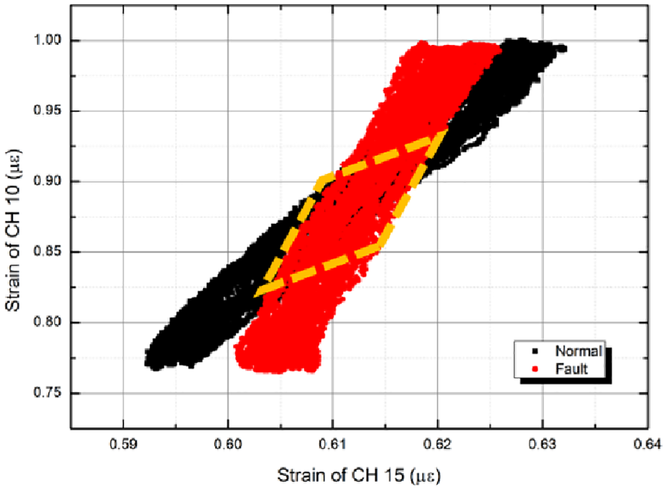
In addition to that based on the original data, fault detection can also be performed using only partial data. The partial data is sampled from the original data from the strain channel CH 10, which is attached to the crack where the accuracy of the decision boundary line was high, and the normal and fault cycles of CH 4, which is a channel attached to the cracked section steel in the damage scenario #2.

Figure 7 shows the plot of the strain data extracted from these two channels. Based on one cycle, only 200 strain data were used at the front and rear based on the maximum peak strain value, which is equal to half the number of data per cycle. The same maximum and minimum strain values from the original data are used in the data normalization process, and the partial normal and fault data are plotted as shown in Figure 6. It is also possible to check whether the maximum or minimum values are included inversely based on the hysteresis of the strain measured in the two channels. A relative slope between the normal and fault regions is also possible if the extreme value is excluded and the slope of the same sign goes from the extreme value to the extreme value, such as the relative slope between the normal and fault regions, and the accuracy calculation of the decision foundation line is performed using machine learning. Figure 6(b) shows the result of extracting 200 strain data at the front and rear based on the damage scenario and the minimum strain value from the channel. It is also possible to check that a partial section is selected in the opposite area; fault detection is possible based on the point data in this area.

Figure 7.

Graphs of partial data extracted as (a) maximum peak strain and near value and (b) minimum peak strain and near value.

Thus, even if the quantity of data is high, reducing the number of data in each feature based on a specific standard would enable the same fault detection method used with the original data to be performed.

Conclusion

In this study, for a truss model assembled with a constant torque using bolts, the variation in the strain due to the inclusion or exclusion of cracks in the section steel under repeated loads is confirmed. The models mounted on the test machine were constructed in a similar manner to the load condition of the mechanical structure used on the actual site, and the results of the strain appearing within the elastic zone and the treatment method were studied. For medium- to large-sized structures, dozens of strain gauges are attached for instrumentation experiments, and machine learning–based logistic regression was used to detect failures based solely on strain data. As a result, when the strain gauge attached to the cracked section steel and that attached to the normal section steel were graphically plotted, the difference in slope was found to differ from that when two strain gauges are attached to normal section steel, which showed a quantitative basis for calculating the accuracy of the decision boundary line. In addition, it was confirmed that the same fault detection method can be applied if the number of data is reduced collectively by plotting the partial strain data.

Footnotes

Appendix

Handling Editor: James Baldwin

Declaration of conflicting interests

The author(s) declared no potential conflicts of interest with respect to the research, authorship, and/or publication of this article.

Funding

The author(s) disclosed receipt of the following financial support for the research, authorship, and/or publication of this article: This work was financially supported by Development of core machinery technologies for Development of Industrial Off-road Working System Technologies Supporting Autonomous Operations (No. NK224H) funded by the Major Institutional Project of Korea Institute of Machinery and Materials (KIMM) and Virtual engineering platform development project (No. MT1290) funded by the Ministry of Trade, Industry and Energy (MOTIE, Korea) and Korea Institute for Advancement of Technology (KIAT).

ORCID iD

Hyejin Bang

References

Bakhtiari-Nejad

Rahai

Esfandiari

A structural damage detection method using static noisy data. Eng Struct 2005; 27: 1784–1793.

Yam

Wong

WO.

Sensitivity studies of parameters for damage detection of plate-like structures using static and dyamic approaches. Eng Struct 2002; 24: 1465–1475.

Rageh

Linzell

Azam

SE.

Automated, strain-based, output-only bridge damage detection. J Civ Struct Health Monit 2018; 8: 8333–8846.

Brunell

Kim

YJ.

Effect of local damage on the behavior of a laboratory-scale steel truss bridge. Eng Struct 2013; 48: 281–291.

Anastasopoulos

De Smedt

Vandewalle

, et al. Damage identification using modal strains identified from operational fiber-optic Bragg grating data. Struct Health Monit 2018; 17: 1441–1459.

Butterfield

Meruane

Collins

, et al. Prediction of leak flow rate in plastic water distribution pipes using vibro-acoustic measurements. Struct Health Monit 2018; 17: 959–970.

Neerukatti

Chattopadhyay

Iyyer

, et al. A hybrid prognosis model for predicting fatigue crack propagation under biaxial in-phase and out-of-phase loading. Struct Health Monit 2018; 17: 888–901.

Eker

Camci

Jennions

IK.

A new hybrid prognostic methodology. Int J Progn Health Manag 2019; 10: 1–10.

Sikorska

Hodkiewicz

Prognostic modelling options for remaining useful life estimation by industry. Mech Syst Signal Process 2010; 25: 1803–1836.

10.

Sanayei

Saletnik

MJ.

Parameter estimation of structures from static strain measurements. I: formulation. J Struct Eng 1996; 122: 555–562.

11.

Liu

Chian

Parametric identification of truss structures using static strains. J Struct Eng 1997; 123: 927–933.

12.

Blachowski

Spencer

, et al. Axial strain accelerations approach for damage localization in statically determinate truss structures. Comput Aided Civ Infrastruct Eng 2017; 32: 304–318.

13.

Bandyopadhyay

Saha

Sohail

Identification of parameter of truss structure by limited static strain measurement. Recent Adv Struct Eng 2019; 1: 375–388.

14.

Farrar

Worden

Structural health monitoring a machine learning perspective. A John Wiley & Sons, Ltd., Publication, 2013, pp.295–399.

15.

Ying

Garrett

Jr Oppenheim

, et al. Toward data-driven structural health monitoring: application of machine learning and signal processing to damage detection. J Comput Civ Eng 2013; 27: 667–680.

16.

Kurian

Liyanapathirana

. Machine learning techniques for structural health monitoring. In: Proceedings of the 13th international conference on damage assessment of structures, Porto, Portugal, 9–10 July 2019, pp.3–24. Singapore: Springer.

17.

Korean Standards Association. Dimensions, mass and permissible variations of hot rolled steel sections, KS D 3502, 2016.

18.

Korean Standards Association. Light gauges steels for general structure, KS D 3530, 2018.