Theoretical study of unsteady oblique stagnation point based Jeffrey nanofluid flow over an oscillatory stretching sheet

Abstract

The numerical analysis for two-dimensional oblique stagnation point flow with the magnetohydrodynamic effects of an incompressible unsteady Jeffrey fluid model caused by an oscillatory and stretching sheet has been presented in this article. The Brownian motion and thermophoresis impacts are taken into consideration. The similarity transformation technique is implemented on the governing partial differential equations of the Jeffrey fluid model to obtain a set of nonlinear coupled ordinary differential equations and then these resulting equations are numerically computed with the help of BVP-Maple programming. The variation in the behavior of velocity, temperature, and concentration profile influenced by the governing parameters, has been explicitly explored and displayed through graphs. The numerical results are highlighted in tabular form and through these outcomes, the skin friction coefficient, Nusselt number, and Sherwood number have been investigated. These physical quantities rise for gradually increasing the Hartmann number and ratio of relaxation to retardation time. However, these reduce for gradually growing Jeffrey fluid parameter.

Introduction

The study of stagnation point flow becomes a very popular field of interest nowadays. Many researchers are exploring the facts of this flow for various types of fluids and for different setups such as orthogonal or nonorthogonal. Several scientists and researchers studied different sorts of surfaces where this phenomenon takes place like stretching, shrinking, lubricated, oscillatory, and many others. The stagnation point flow was first investigated by Hiemenz. ¹ He studied the boundary layer procedure for a fluid flow towards an obstacle and a straight wall as well. He implemented a similarity transformation method on the mathematical fluid model and attained a series solution. Later, this model was investigated by Howarth ² for three dimensions. Rott ³ considered steady orthogonal stagnation flow. The non-orthogonal case was first explored by Stuart. ⁴ A mathematical fluid model for oblique stagnation flow was evaluated by Tamada. ⁵ Mahapatra and Gupta ⁶ investigated the MHD flow at the stretching sheet under the stagnation point region. Akbar et al. ⁷ discussed the MHD flow of nanofluid at the stretching surface under the stagnation point region. They found the results of radiation effects and convective boundary conditions at the stretching sheet. Rehman et al. ⁸ investigated the heat and mass transfer of the nonlinear stretching surface under the stagnation point region. Besthapu et al. ⁹ highlighted the impact of slip and thermal radiation on the nonlinear stretching sheet under the stagnation point region. Few authors have been discussed the stagnation flow at a stretching surface under various assumptions see Nadeem et al. ¹⁰ and Waini et al. ¹¹ Choi and Eastman ¹² provided the concept of nanofluids which became very valuable in many applications in the industry because nanofluids are very effective for increment in thermal conductivity. Buongiorno ¹³ took the influence of Brownian motion and thermophoresis into consideration and created a fluid model incorporated with these effects. Stagnation point flow was investigated by Mahapatra and Gupta ¹⁴ for viscoelastic fluid over a flat deformable sheet. An important result of oblique stagnation point flow with MHD effects was deduced by Borrelli et al.^15,16 The oblique stagnation flow takes place if and only if the applied magnetic field and dividing streamlines are in the same direction. A model of second-grade fluid with the well known Buongiorno model was provided by Nadeem et al., ¹⁷ the results indicated that the stretching velocity has an impact on the formulation of the boundary layer. Khan et al. ¹⁸ investigated a series solution technique to observe the oblique stagnation point flow for the viscous nanofluid along with the slip and magnetic impacts. Flow and heat transfer investigation was taken into the account by Mehmood et al. ¹⁹ for the stagnation point flow of the Jeffrey nanofluid model which was obliquely hitting the stretched plate and involved with the Buongiorno model. The stagnation point flow was explored on a curved surface by Nadeem et al. ²⁰ The dual solutions for an oscillatory shrinking and stretching sheet were attained by Nadeem et al. ²¹ Nadeem et al. ²² evaluated results for micropolar nanofluid with magnetic and slip impacts, where the surface was stretching and oscillatory and taken in a porous medium. Nanofluid flow discussed by authors (see the Saif et al. ²³ and Haq et al. ²⁴ ) for different assumptions.

Ahmed ²⁵ obtained non-similar solutions for the natural convection boundary layer flow of a micropolar nanofluid on to a vertical permeable cone with variable wall temperatures. Ahmed^26–28 provided the results for nanofluid flows in inclined enclosures for the porous medium. Ahmed ²⁹ analyzed a dusty hybrid nanofluid flow in wavy enclosures containing a volumetric heat source and utilized the SIMPLE techniques to obtain the pressure terms for both the considered nanofluid and dusty particles based on the control volume solver. Hsiao ³⁰ examined the stagnation nano energy conversion problems for conjugate mixed convection heat and mass transfer with EMHD effects on to a stretching surface. The energy conversion problem was investigated by Hsiao^31–33 for non-Newtonian fluids with magnetic effects in order to observe the heat transfer enhancement.

This current research work is concerned with the analysis of oblique stagnation point flow with the MHD impacts of Jeffrey fluid model on to an oscillatory and stretching sheet. The impacts of Brownian motion and thermophoresis are also included. The governing PDEs have been derived for Jeffrey fluid and a similarity transformation method is applied to convert these equations into a set of nonlinear coupled ODEs. The resulting equations have been numerically solved through the use of BVP-Maple software. Graphical and tabular results are presented with the aim of interpreting the behavior of concentration, temperature, velocity fields, Nusselt number, skin friction coefficient, and Sherwood number, in the consequence of variation in governing parameters. Nobody has evaluated the combined effects of MHD oblique stagnation point flow for the Jeffrey fluid on to an oscillatory stretching sheet with Brownian motion and thermophoresis effects. The involved parameters for heat and mass transfer are discussed for both the cases of stretching parameter for less and greater than one. Therefore, the results of the present work are new in literature.

Mathematical formulation

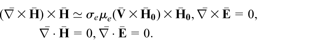
Let us consider an unsteady oblique stagnation point flow of an incompressible Jeffrey fluid with magnetohydrodynamic effects, caused by a sheet which is supposed as oscillatory and stretching. This sheet is oscillating harmonically in its own plane with velocity $U_0\cos \omega \overline{t}$ and the stretching velocity is $c\overline{x}$ . The flow is considered in two dimensions where the fluid is striking obliquely to the surface $\overline{y}=A_p$ and a uniform magnetic field of strength $B_0$ is applied parallel to the dividing streamlines, where the effect of induced magnetic field is negligible as $\overline{\mathbf{E}}=0$ . The Maxwell’s equations for the magnetic field are as follows,

$$\begin{array}{c}\multicolumn{1}{c}{(\overline{\nabla }\times \overline{\mathbf{H}})\times \overline{\mathbf{H}}\simeq {\sigma }_e{\mu }_e(\overline{\mathbf{V}}\times {\overline{\mathbf{H}}}_0)\times {\overline{\mathbf{H}}}_0,\overline{\nabla }\times \overline{\mathbf{E}}=0,}\\ \multicolumn{1}{c}{\overline{\nabla }·\overline{\mathbf{H}}=0,\overline{\nabla }·\overline{\mathbf{E}}=0.}\end{array}$$

Where $B_0={\mu }_e{H}_0$ and the external magnetic field is ${\overline{\mathbf{H}}}_0=\frac{H_0}{\sqrt{4a^2+b^2}}(-b\hat{i}+2a\hat{j})$ , as reported by Borrelli et al. ¹⁶ The effects of thermophoresis and Brownian motion are also considered. Schematic diagram of the considered problem is presented in the Figure 1.

Figure 1.

Geometry of the problem.

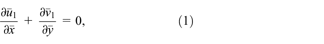
The governing flow field equations are given as follows,

$$\frac{\partial {\overline{u}}_1}{\partial \overline{x}}+\frac{\partial {\overline{v}}_1}{\partial \overline{y}}=0,$$

(1)

$$\begin{array}{c}\frac{\partial {\overline{u}}_1}{\partial \overline{t}}+{\overline{u}}_1\frac{\partial {\overline{u}}_1}{\partial \overline{x}}+{\overline{v}}_1\frac{\partial {\overline{u}}_1}{\partial \overline{y}}=-\frac{1}{\rho }\frac{\partial \overline{p}}{\partial \overline{x}}+\frac{\nu }{1+{\lambda }_1}[(\frac{{\partial }^2{\overline{u}}_1}{\partial {\overline{x}}^2}+\frac{{\partial }^2{\overline{u}}_1}{\partial {\overline{y}}^2})+2{\lambda }_2\frac{\partial }{\partial \overline{x}}({\overline{u}}_1\frac{{\partial }^2{\overline{u}}_1}{\partial {\overline{x}}^2}+{\overline{v}}_1\frac{{\partial }^2{\overline{u}}_1}{\partial \overline{x}\partial \overline{y}})\hfill \\ +{\lambda }_2\frac{\partial }{\partial \overline{y}}\{{\overline{u}}_1(\frac{{\partial }^2{\overline{u}}_1}{\partial \overline{x}\partial \overline{y}}+\frac{{\partial }^2{\overline{v}}_1}{\partial {\overline{x}}^2})+{\overline{v}}_1(\frac{{\partial }^2{\overline{v}}_1}{\partial \overline{x}\partial \overline{y}}+\frac{{\partial }^2{\overline{u}}_1}{\partial {\overline{y}}^2})\}]-4a^2\frac{\sigma }{\rho }\frac{{(B_0)}^2{\overline{u}}_1}{4a^2+b^2},\hfill \end{array}$$

(2)

$$\begin{array}{c}\frac{\partial {\overline{v}}_1}{\partial \overline{t}}+{\overline{u}}_1\frac{\partial {\overline{v}}_1}{\partial \overline{x}}+{\overline{v}}_1\frac{\partial {\overline{v}}_1}{\partial \overline{y}}=-\frac{1}{\rho }\frac{\partial \overline{p}}{\partial \overline{y}}+\frac{\nu }{1+{\lambda }_1}[(\frac{{\partial }^2{\overline{v}}_1}{\partial {\overline{x}}^2}+\frac{{\partial }^2{\overline{v}}_1}{\partial {\overline{y}}^2})+{\lambda }_2\frac{\partial }{\partial \overline{x}}\{{\overline{u}}_1(\frac{{\partial }^2{\overline{v}}_1}{\partial {\overline{x}}^2}+\frac{{\partial }^2{\overline{u}}_1}{\partial \overline{y}\partial \overline{x}})\hfill \\ +{\overline{v}}_1(\frac{{\partial }^2{\overline{u}}_1}{\partial {\overline{y}}^2}+\frac{{\partial }^2{\overline{v}}_1}{\partial \overline{x}\partial \overline{y}})\}+2{\lambda }_2\frac{\partial }{\partial \overline{y}}({\overline{u}}_1\frac{{\partial }^2{\overline{v}}_1}{\partial \overline{y}\partial \overline{x}}+{\overline{v}}_1\frac{{\partial }^2{\overline{v}}_1}{\partial {\overline{y}}^2})]-4a^2\frac{\sigma }{\rho }\frac{{(B_0)}^2{\overline{v}}_1}{4a^2+b^2},\hfill \end{array}$$

(3)

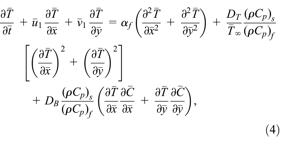
The energy and concentration equations as reported in Buongiorno ¹³ are given as,

$$\begin{array}{c}\frac{\partial \overline{T}}{\partial \overline{t}}+{\overline{u}}_1\frac{\partial \overline{T}}{\partial \overline{x}}+{\overline{v}}_1\frac{\partial \overline{T}}{\partial \overline{y}}={\alpha }_f(\frac{{\partial }^2\overline{T}}{\partial {\overline{x}}^2}+\frac{{\partial }^2\overline{T}}{\partial {\overline{y}}^2})+\frac{D_T}{{\overline{T}}_{\infty }}\frac{{(\rho C_p)}_s}{{(\rho C_p)}_f}\hfill \\ \multicolumn{1}{c}{[{\left(\frac{\partial \overline{T}}{\partial \overline{x}}\right)}^2+{\left(\frac{\partial \overline{T}}{\partial \overline{y}}\right)}^2]}\\ +D_B\frac{{(\rho C_p)}_s}{{(\rho C_p)}_f}(\frac{\partial \overline{T}}{\partial \overline{x}}\frac{\partial \overline{C}}{\partial \overline{x}}+\frac{\partial \overline{T}}{\partial \overline{y}}\frac{\partial \overline{C}}{\partial \overline{y}}),\hfill \end{array}$$

(4)

$$\frac{\partial \overline{C}}{\partial \overline{t}}+{\overline{u}}_1\frac{\partial \overline{C}}{\partial \overline{x}}+{\overline{v}}_1\frac{\partial \overline{C}}{\partial \overline{y}}=\frac{D_T}{{\overline{T}}_{\infty }}(\frac{{\partial }^2\overline{T}}{\partial {\overline{x}}^2}+\frac{{\partial }^2\overline{T}}{\partial {\overline{y}}^2})+D_B(\frac{{\partial }^2\overline{C}}{\partial {\overline{x}}^2}+\frac{{\partial }^2\overline{C}}{\partial {\overline{y}}^2}).$$

(5)

Let $\mathrm{\Delta }\overline{T}={\overline{T}}_w-{\overline{T}}_{\infty }$ be the difference between reference and ambient temperature and $\mathrm{\Delta }\overline{C}={\overline{C}}_w-{\overline{C}}_{\infty }$ be the difference between reference and ambient concentration.

The boundary conditions for equation (1) to (5) are as follows

$$\begin{array}{c}{\overline{u}}_1=c\overline{x}+U_0\cos \omega \overline{t},{\overline{v}}_1=-{\overline{v}}_w,\overline{T}={\overline{T}}_w\hfill \\ \multicolumn{1}{c}{+ϵ\mathrm{\Delta }\overline{T}\mathrm{Re}[e^{\stackrel{·}{\iota }\omega \overline{t}}],\overline{C}={\overline{C}}_w+ϵ\mathrm{\Delta }\overline{C}\mathrm{Re}[e^{\stackrel{·}{\iota }\omega \overline{t}}],\mathrm{at}\overline{y}=0,}\\ \multicolumn{1}{c}{{\overline{u}}_1=a\overline{x}+b(\overline{y}-B_p),{\overline{v}}_1=-a(\overline{y}-A_p),\overline{T}={\overline{T}}_{\infty },}\\ \multicolumn{1}{c}{\overline{C}={\overline{C}}_{\infty },\mathrm{as}\overline{y}\to \infty .}\end{array}\}$$

(6)

The conditions ${\overline{u}}_1=a\overline{x}+b(\overline{y}-B_p)$ and ${\overline{v}}_1=-a(\overline{y}-A_p)$ in (6) indicate that the stagnation point is at $(\frac{b}{a}(B_p-A_p),A_p)$ . The streamlines are hyperbolas whose asymptotes are given as

$$\overline{y}=A_p\mathrm{and}\overline{y}=-\frac{2a}{b}\overline{x}+2B_p-A_p.$$

Let us suppose the components of velocity as

$${\overline{u}}_1=a\overline{x}\overline{F}\prime (\overline{y})+b\overline{G}(\overline{y},\overline{t})\mathrm{and}{\overline{v}}_1=-a\overline{F}(\overline{y}).$$

(7)

These velocity components are substituted in governing equations. The pressure field is eliminated by comparison of equation (2) and equation (3) using ${\overline{p}}_{\overline{x}\overline{y}}={\overline{p}}_{\overline{y}\overline{x}}$ .

The flow equations took the form

$$\begin{array}{c}\multicolumn{1}{c}{\overline{F}\overline{F}″-\overline{F}{\prime }^2+\frac{1}{a}\left(\frac{\nu }{1+{\lambda }_1}\right)[\overline{F}″\prime +a{\lambda }_2\{\overline{F}\prime {\prime }^2-\overline{F}{\overline{F}}^{\mathrm{iv}}\}]}\\ \multicolumn{1}{c}{+\left(4a\frac{\sigma }{\rho }\frac{B_0^2}{4a^2+b^2}\right)(1-\overline{F}\prime )+1=0,}\end{array}$$

(8)

$$\begin{array}{c}\overline{F}\overline{G}\prime -\overline{G}\overline{F}\prime -\frac{1}{a}{\overline{G}}_{\overline{t}}+\frac{1}{a}\left(\frac{\nu }{1+{\lambda }_1}\right)\hfill \\ \multicolumn{1}{c}{[\overline{G}″+a{\lambda }_2\{\overline{G}\overline{F}″\prime +\overline{G}\prime \overline{F}″-\overline{F}\overline{G}″\prime -\overline{F}\prime \overline{G}″\}}\\ +\left(4a\frac{\sigma }{\rho }\frac{B_0^2}{4a^2+b^2}\right)(\overline{F}-\overline{G})\hfill \\ \multicolumn{1}{c}{-(1+4a\frac{\sigma }{\rho }\frac{B_0^2}{4a^2+b^2})(B_p-A_p)=0.}\end{array}$$

(9)

The boundary conditions (6) become

$$\begin{array}{c}\multicolumn{1}{c}{\overline{F}(0)=\frac{v_w}{a},\overline{F}\prime (0)=\frac{c}{a},\overline{G}(0,\overline{t})=\mathrm{Re}\left[\frac{U}{b}{e}^{\stackrel{·}{\iota }\omega \overline{t}}\right],}\\ \multicolumn{1}{c}{\overline{F}\prime (\infty )=1,\overline{G}\prime (\infty ,\overline{t})=1.}\end{array}$$

(10)

From (10), the asymptotic solution of $\overline{F}$ and $\overline{G}$ is given as

$$\overline{F}~\overline{y}-A_p\mathrm{and}\overline{G}~\overline{y}-B_p,\mathrm{as}\overline{y}\to \infty .$$

The dimensionless variables are assumed as

$$\begin{array}{c}t=\omega \overline{t},y=\sqrt{\frac{a}{\nu }}\overline{y},F(y)=\sqrt{\frac{a}{\nu }}\overline{F}(\overline{y}),G_0(y)+ϵG_1(y)e^{\stackrel{·}{\iota }t}\hfill \\ \multicolumn{1}{c}{=\sqrt{\frac{a}{\nu }}\overline{G}(\overline{y},\overline{t}),}\\ \multicolumn{1}{c}{\theta (t,y)=[{\theta }_0(y)+ϵ{\theta }_1(y)e^{\stackrel{·}{\iota }t}]=\frac{\overline{T}-{\overline{T}}_{\infty }}{\mathrm{\Delta }\overline{T}},}\\ \multicolumn{1}{c}{\varphi (t,y)=[{\varphi }_0(y)+ϵ{\varphi }_1(y)e^{\stackrel{·}{\iota }t}]=\frac{\overline{C}-{\overline{C}}_{\infty }}{\mathrm{\Delta }\overline{C}}.}\end{array}\}$$

(11)

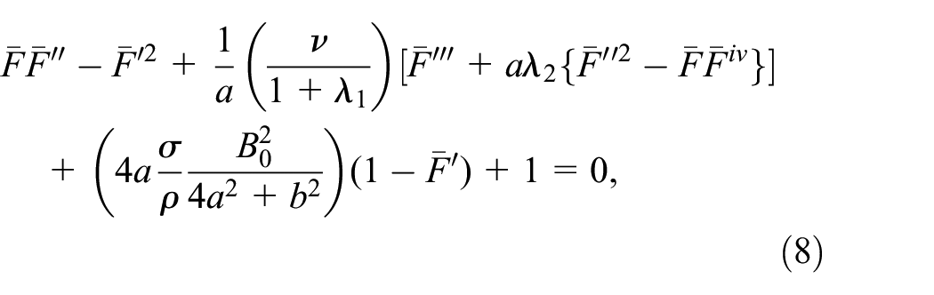
The dimensionless form of flow field equations is obtained by utilizing (11) and it is given as follows

$$\begin{array}{c}\multicolumn{1}{c}{\mathrm{FF}″-F{\prime }^2+\left(\frac{1}{1+{\lambda }_1}\right)[F″\prime +K\{{F″}^2-F{F}^{\mathrm{iv}}\}]}\\ \multicolumn{1}{c}{+M^2(1-F\prime )+1=0,}\end{array}$$

(12)

$$\begin{array}{c}\mathrm{FG}{\prime }_0-G_{0}F\prime +\left(\frac{1}{1+{\lambda }_1}\right)\hfill \\ \multicolumn{1}{c}{[G_0^{″}+K\{G_{0}F″\prime +G_0^{\prime }F″-{\mathrm{FG}}_0^{″\prime }-F\prime G_0^{″}\}]}\\ +M^2(F-G_0)-(1+M^2)(\mathbb{B}-\mathbb{A})=0,\hfill \end{array}$$

(13)

$$\begin{array}{c}\multicolumn{1}{c}{\mathrm{FG}{\prime }_1-G_{1}F\prime -\mathrm{\Omega }\stackrel{·}{\iota }{G}_1+\left(\frac{1}{1+{\lambda }_1}\right)}\\ \multicolumn{1}{c}{[G_1^{″}+K\{G_{1}F″\prime +G_1^{\prime }F″-{\mathrm{FG}}_1^{″\prime }-F\prime G_1^{″}\}]-M^2{G}_1=0,}\end{array}$$

(14)

$$\frac{1}{\mathrm{Pr}}{\theta }_0^{″}+F{\theta }_0^{\prime }+\mathrm{Nb}({\theta }_0^{\prime }{\varphi }_0^{\prime })+\mathrm{Nt}({\theta }_0^{\prime }{)}^2=0,$$

(15)

$$\frac{1}{\mathrm{Pr}}{\theta }_1^{″}+F{\theta }_1^{\prime }-\stackrel{·}{\iota }\mathrm{\Omega }{\theta }_1+\mathrm{Nb}({\theta }_0^{\prime }{\varphi }_1^{\prime }+{\theta }_1^{\prime }{\varphi }_0^{\prime })+2\mathrm{Nt}({\theta }_0^{\prime }{\theta }_1^{\prime })=0,$$

(16)

$${\varphi }_0^{″}+\mathrm{Sc}(F{\varphi }_0^{\prime })+\frac{\mathrm{Nt}}{\mathrm{Nb}}{\theta }_0^{″}=0,$$

(17)

$${\varphi }_1^{″}+\mathrm{Sc}(F{\varphi }_0^{\prime }-\stackrel{·}{\iota }\mathrm{\Omega }{\varphi }_1)+\frac{\mathrm{Nt}}{\mathrm{Nb}}{\theta }_1^{″}=0,$$

(18)

with the conditions

$$\begin{array}{c}F(0)=S,F\prime (0)=\gamma ,G_0(0)=0,G_1(0)=1,\hfill \\ \multicolumn{1}{c}{{\theta }_0(0)=1,{\theta }_1(0)=1,{\varphi }_0(0)=1,{\varphi }_1(0)=1,}\\ \multicolumn{1}{c}{F\prime (y)=1,G_0^{\prime }(y)=1,G_1^{\prime }(y)=0,{\theta }_0(y)=0,}\\ \multicolumn{1}{c}{{\theta }_1(y)=0,{\varphi }_0(y)=0,{\varphi }_1(y)=0,}\\ \multicolumn{1}{c}{F~y-\mathbb{A}\mathrm{and}G~y-\mathbb{B},\mathrm{as}y\to \infty ,}\end{array}\}$$

(19)

where

$$\begin{array}{c}K=a{\lambda }_2,\mathbb{A}=\sqrt{\frac{a}{\nu }}{A}_p,\mathbb{B}=\sqrt{\frac{a}{\nu }}{B}_p,\mathrm{Nt}=\frac{D_T}{T_{\infty }}\frac{{(\rho C_p)}_s}{{(\rho C_p)}_f}\frac{\mathrm{\Delta }\overline{T}}{\nu },\hfill \\ \multicolumn{1}{c}{\mathrm{Nb}=D_B\frac{{(\rho C_p)}_s}{{(\rho C_p)}_f}\frac{\mathrm{\Delta }\overline{C}}{\nu },}\\ M^2=4a\frac{\sigma }{\rho }\frac{B_0^2}{4a^2+b^2},ϵ=\sqrt{\frac{a}{\nu }}\frac{U_0}{b},\mathrm{\Omega }=\frac{\omega }{a},\mathrm{Pr}=\frac{\nu }{{\alpha }_f},\hfill \\ \multicolumn{1}{c}{\gamma =\frac{c}{a},S=\frac{{\nu }_w}{\sqrt{a\nu }},\mathrm{Sc}=\frac{\nu }{D_B}.}\end{array}$$

${\lambda }_1$ is ratio of relaxation to retardation time, ${\lambda }_2$ is retardation time, $K$ is Jeffrey fluid parameter, $\gamma$ is stretching parameter, $\mathrm{Nb}$ is Brownian motion parameter, $\mathrm{Nt}$ is thermophoresis parameter, $S$ is suction parameter, $\mathrm{Pr}$ is Prandtl number, $M$ is Hartmann number, and $\mathrm{Sc}$ is Schmidt number.

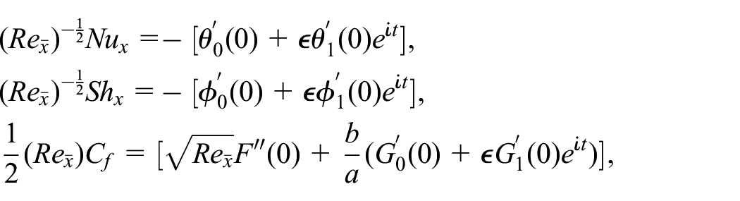
The Nusselt number $N{u}_x$ , Sherwood number $S{h}_x$ , skin friction coefficient $C_f$ , local heat flux $q_w$ , mass diffusion flux $j_w$ , and local surface shear stress ${\tau }_w$ are represented as follows

$$\begin{array}{c}N{u}_x=\frac{\overline{x}{q}_w}{k\mathrm{\Delta }\overline{T}},S{h}_x=\frac{\overline{x}{j}_w}{D\mathrm{\Delta }\overline{C}},C_f=\frac{{\tau }_w}{\frac{1}{2}\rho U_w^2},\hfill \\ q_w=-k\frac{\partial \overline{T}}{\partial \overline{y}}{|}_{\overline{y}=0},j_w=-D\frac{\partial \overline{C}}{\partial \overline{y}}{|}_{\overline{y}=0},{\tau }_w=-\mu \frac{\partial {\overline{u}}_1}{\partial \overline{y}}{|}_{\overline{y}=0}.\hfill \end{array}$$

With the help of similarity variables (11), the above relations took the form as

$$\begin{array}{c}(R{e}_{\overline{x}}{)}^{-\frac{1}{2}}N{u}_x=-[{\theta }_0^{\prime }(0)+ϵ{\theta }_1^{\prime }(0)e^{\stackrel{·}{\iota }t}],\hfill \\ (R{e}_{\overline{x}}{)}^{-\frac{1}{2}}S{h}_x=-[{\varphi }_0^{\prime }(0)+ϵ{\varphi }_1^{\prime }(0)e^{\stackrel{·}{\iota }t}],\hfill \\ \frac{1}{2}(R{e}_{\overline{x}})C_f=[\sqrt{R{e}_{\overline{x}}}F″(0)+\frac{b}{a}(G_0^{\prime }(0)+ϵG_1^{\prime }(0)e^{\stackrel{·}{\iota }t})],\hfill \end{array}$$

where local Reynolds number can be expressed as $R{e}_{\overline{x}}=\frac{a{x}^2}{\nu }$ .

The stagnation point $\overline{x}=0$ , the point of maximum pressure $\overline{x}={\overline{x}}_p$ and the point of zero skin friction $\overline{x}={\overline{x}}_s$ are the three main points at the surface. The stagnation point is derived from

$$\begin{array}{c}\multicolumn{1}{c}{\mathrm{xF}(y)+\frac{b}{a}({\int }_0^y{G}_0(s)\mathrm{ds}+ϵe^{\stackrel{·}{\iota }t}{\int }_0^y{G}_1(s)\mathrm{ds})=0,}\\ \multicolumn{1}{c}{x=\sqrt{\frac{a}{\nu }}\overline{x}.}\end{array}$$

At the point of maximum pressure, the fluid velocity becomes zero. From the conditions ${\overline{u}}_1=a\overline{x}+b(\overline{y}-B_p)$ and ${\overline{v}}_1=-a(\overline{y}-A_p)$ in (6), the pressure can be obtained by using ${\overline{u}}_1={\overline{v}}_1=0$ . Therefore, the point of maximum pressure ${\overline{x}}_p$ is given as

$${\overline{x}}_p=(\mathbb{B}-\mathbb{A})\frac{b}{a}\sqrt{\frac{\nu }{a}}.$$

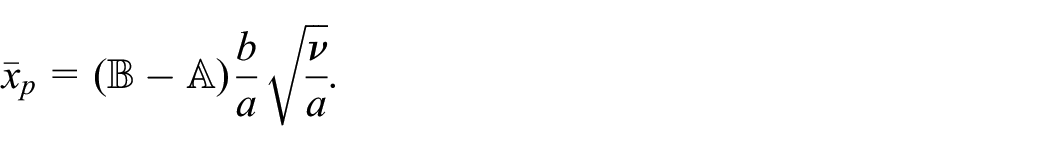
The point of zero skin friction ${\overline{x}}_s$ is given as

$${\overline{x}}_s=-\frac{b}{a}\sqrt{\frac{\nu }{a}}\frac{(G_0^{\prime }(0)+ϵG_1^{\prime }(0)e^{\stackrel{·}{\iota }t})}{F″(0)}.$$

The ratio $\frac{{\overline{x}}_p}{{\overline{x}}_s}$ is same for all angle of incidence, that is

$$\frac{{\overline{x}}_p}{{\overline{x}}_s}=-(\mathbb{B}-\mathbb{A})\frac{F″(0)}{(G_0^{\prime }(0)+ϵG_1^{\prime }(0)e^{\stackrel{·}{\iota }t})}.$$

Solution procedure

The equations (12), (13), (15), and (17) along with their boundary conditions (19) have been numerically solved utilizing BVP solution method in Maple software. The series solutions of equations (14), (16), and (18) have been obtained for the small values of frequency parameter $\mathrm{\Omega }$ .

$$G_1(y)=\sum _{n=0}^{n=\infty }(\stackrel{·}{\iota }\mathrm{\Omega }{)}^n{H}_n(y),$$

$${\theta }_1(y)=\sum _{n=0}^{n=\infty }(\stackrel{·}{\iota }\mathrm{\Omega }{)}^n{\theta }_{1n}(y),$$

and

$${\varphi }_1(y)=\sum _{n=0}^{n=\infty }(\stackrel{·}{\iota }\mathrm{\Omega }{)}^n{\varphi }_{1n}(y).$$

The real part of these solutions are given as

$$G_1(y)=H_0(y)-{\mathrm{\Omega }}^2{H}_2(y)+{\mathrm{\Omega }}^4{H}_4(y)-\dots ,$$

$${\theta }_1(y)={\theta }_{10}(y)-{\mathrm{\Omega }}^2{\theta }_{12}(y)+{\mathrm{\Omega }}^4{\theta }_{14}(y)-\dots ,$$

and

$${\varphi }_1(y)={\varphi }_{10}(y)-{\mathrm{\Omega }}^2{\varphi }_{12}(y)+{\mathrm{\Omega }}^4{\varphi }_{14}(y)-\dots .$$

The equation (14) reduces to

$$\begin{array}{c}{\mathrm{FH}}_0^{\prime }-H_{0}F\prime +(\frac{1}{1+{\lambda }_1})[H_0^{″}+K\{H_{0}F″\prime +H_0^{\prime }F″-{\mathrm{FH}}_0^{″\prime }\hfill \\ \multicolumn{1}{c}{-F\prime H_0^{″}\}]-M^2{H}_0=0,}\\ \multicolumn{1}{c}{{\mathrm{FH}}_n^{\prime }-H_{n}F\prime +(\frac{1}{1+{\lambda }_1})[H_n^{″}+K\{H_{n}F″\prime +H_n^{\prime }F″-{\mathrm{FH}}_n^{″\prime }}\\ \multicolumn{1}{c}{-F\prime H_n^{″}\}]-M^2{H}_n-H_{n-1}=0,}\\ \multicolumn{1}{c}{H_0(0)=1,H_0(\infty )=0,H_n(0)=0,H_n(\infty )=0,}\\ \multicolumn{1}{c}{n=1,2,3,\dots }\end{array}\}$$

and Equations (16) and (18) reduce to

$$\begin{array}{c}\frac{1}{\mathrm{Pr}}{\theta }_{10}^{″}+F{\theta }_{10}^{\prime }+\mathrm{Nb}({\theta }_0^{\prime }{\varphi }_{10}^{\prime }+{\theta }_{10}^{\prime }{\varphi }_0^{\prime })+2\mathrm{Nt}({\theta }_0^{\prime }{\theta }_{10}^{\prime })=0,\hfill \\ \multicolumn{1}{c}{\frac{1}{\mathrm{Pr}}{\theta }_{1n}^{″}+F{\theta }_{1n}^{\prime }+\mathrm{Nb}({\theta }_0^{\prime }{\varphi }_{1n}^{\prime }+{\theta }_{1n}^{\prime }{\varphi }_0^{\prime })+2\mathrm{Nt}({\theta }_0^{\prime }{\theta }_{1n}^{\prime })}\\ \multicolumn{1}{c}{-{\theta }_{1(n-1)}=0,}\\ \multicolumn{1}{c}{{\varphi }_{10}^{″}+\mathrm{Sc}(F{\varphi }_0^{\prime })+\frac{\mathrm{Nt}}{\mathrm{Nb}}{\theta }_{10}^{″}=0,}\\ \multicolumn{1}{c}{{\varphi }_{1n}^{″}+\mathrm{Sc}(F{\varphi }_0^{\prime }-{\varphi }_{1(n-1)})+\frac{\mathrm{Nt}}{\mathrm{Nb}}{\theta }_{1n}^{″}=0,}\\ \multicolumn{1}{c}{{\theta }_{10}(0)=1,{\theta }_{10}(\infty )=0,{\theta }_{1n}(0)=1,{\theta }_{1n}(\infty )=0,}\\ \multicolumn{1}{c}{{\varphi }_{10}(0)=1,{\varphi }_{10}(\infty )=0,{\varphi }_{1n}(0)=1,{\varphi }_{1n}(\infty )=0,}\\ \multicolumn{1}{c}{n=1,2,3,\dots .}\end{array}\}$$

Results and discussion

The equations (12) to (18) with their associated boundary conditions (19) have been numerically computed with the help of Maple software. This section concerns with the graphical representation of variations in velocity $F\prime (y)$ , concentration $\varphi (y)$ and temperature $\theta (y)$ profiles caused by the governing physical parameters of the considered fluid flow. These are Hartmann number $M$ , Jeffrey fluid parameter $K$ , suction parameter $S$ , the ratio of relaxation to retardation time ${\lambda }_1$ , Brownian motion parameter $\mathrm{Nb}$ , stretching parameter $\gamma$ , Schmidt number $\mathrm{Sc}$ , thermophoresis parameter $\mathrm{Nt}$ , and Prandtl number $\mathrm{Pr}$ . The physical quantities Sherwood number $S{h}_x$ , coefficient of skin friction $C_f$ , and Nusselt number $N{u}_x$ are investigated through numerical outcomes which are highlighted in tables.

Plots for $F(y)$ , velocity component $F\prime (y)$ , and its gradient $F″(y)$ are depicted in Figure 2 for some fixed values of involved parameters, that is, $M=1.0$ , $K=0.2$ , ${\lambda }_1=0.1$ , and $\mathbb{B}=-5$ .

Figure 2.

Plots showing $F(y)$ , $F\prime (y)$ , and $F″(y)$ for $M=1.0$ , $K=0.2$ , ${\lambda }_1=0.1$ , and $\mathbb{B}=-5$ .

Figure 3 illustrates that how the velocity profile $F\prime (y)$ varies with variation in $M$ , $S$ , $\gamma$ , ${\lambda }_1$ and $K$ . The impact of stretching parameter $\gamma$ is very significant in this flow as the behavior of $F\prime (y)$ is found opposite for $\gamma >1$ and $\gamma <1$ . Results of other parameters $M$ , $S$ , ${\lambda }_1$ and $K$ are opposite when these vary with fixed $\gamma >1$ and $\gamma <1$ . In Figure 3(a), (b), and (d), the variations of $M$ , ${\lambda }_1$ , $S$ (respectively) are considered to determine the behavior of $F\prime (y)$ . The increasing behavior is indicated when $M$ , ${\lambda }_1$ and $S$ increase with $\gamma <1$ while decreasing behavior is revealed when $M$ , ${\lambda }_1$ and $S$ increase with $\gamma >1$ . Figure 3(c) portrays the decreasing behavior of $F\prime (y)$ for variation in $K$ with $\gamma <1$ and depicts the increasing behavior of $F\prime (y)$ for variation in $K$ with $\gamma >1$ . Figure 3(e) displays the variation in $F\prime (y)$ for $\gamma =0.4,0.6,0.8,1.0,1.2,1.4,1.6$ with other fixed parameters.

Figure 3.

Plots for $F\prime (y)$ against: (a) $M$ , (b) ${\lambda }_1$ , (c) $K$ , (d) $S$ , and (e) $\gamma$ .

The behavior of velocity profiles $G_0(y)$ is portrayed in Figure 4. For $G_0(y)$ , value of $\mathbb{B}$ plays a significant role, as the results for positive values of $\mathbb{B}$ appear to be opposite than the negative value of $\mathbb{B}$ . The streamlines will be more oblique towards the left side of the stagnation point when $\mathbb{B}$ increases. Increment in $M$ , ${\lambda }_1$ and $S$ with fixed $\mathbb{B}<0$ causes a rise in $G_0(y)$ . On the other hand, these parameters with fixed $\mathbb{B}>0$ cause a reduction in $G_0(y)$ . $G_0(y)$ shows the decreasing behavior when $K$ increases with fixed $\mathbb{B}<0$ and it is shown in Figure 4(c).

Figure 4.

Plots for $G_0(y)$ against: (a) $M$ , (b) ${\lambda }_1$ , (c) $K$ , and (d) $S$ .

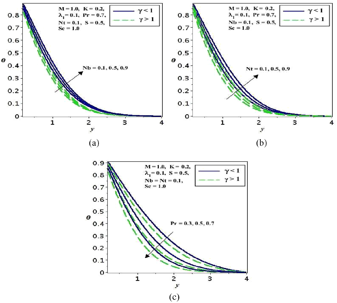
The variations in temperature profile $\theta (y)$ due to the influence of parameters $M$ , $S$ , $\gamma$ , $\mathrm{Nt}$ , $\mathrm{Nb}$ and $\mathrm{Pr}$ are portrayed in Figures 5 and 6. It is detected from Figure 5(a) that $\theta (y)$ decreases when $M$ is increasing with fixed $\gamma <1$ but $\theta (y)$ profile appears to be reverse when increasing $M$ is taken with fixed $\gamma >1$ . Figure 5(b) displays that the $\theta (y)$ profile decreases with higher values of parameter $S$ for both fixed $\gamma <1$ and $\gamma >1$ . Increasing parameter $\gamma$ tends to decrease $\theta (y)$ gradually, this result is depicted in Figure 5(c).

Figure 5.

Plots for temperature profile $\theta (y)$ against: (a) $M$ , (b) $S$ , and (c) $\gamma$ .

Figure 6.

Plots for temperature profile $\theta (y)$ against: (a) $\mathrm{Nb}$ , (b) $\mathrm{Nt}$ , and (c) $\mathrm{Pr}$ .

Figure 6 displays the graphical results for variations in temperature due to increment in parameters $\mathrm{Nb}$ , $\mathrm{Nt}$ and $\mathrm{Pr}$ . The graphs show that the increasing $\mathrm{Nb}$ and $\mathrm{Nt}$ are responsible for the increase in temperature and increasing $\mathrm{Pr}$ causes to decrease the temperature profile. These results are observed in both $\gamma <1$ and $\gamma >1$ cases and displayed in (Figure 6(a)–(c)) respectively.

The influence of parameters $M$ , $S$ , $\gamma$ , $\mathrm{Nt}$ , $\mathrm{Nb}$ and $\mathrm{Sc}$ on concentration profile $\varphi (y)$ is sketched in Figures 7 and 8. The variations in $\varphi (y)$ profile in consequence of increment in parameters $M$ , $S$ and $\gamma$ are shown in Figure 7. Figure 7(a) exhibits the decreasing response of $\varphi (y)$ in the result of increase in $M$ with $\gamma <1$ , on the other hand an increase in $\varphi (y)$ profile can be seen with increase in $M$ with $\gamma >1$ . Figure 7(b) presents that, gradually increasing values of $S$ tend to decrease $\varphi (y)$ profile for both $\gamma <1$ and $\gamma >1$ . Figure 7(c) shows the behavior of $\varphi (y)$ is decreasing, caused by increment in $\gamma$ .

Figure 7.

Plots for temperature profile $\theta (y)$ against: (a) $M$ , (b) $S$ , and (c) $\gamma$ .

Figure 8.

Plots for concentration profile $\varphi (y)$ against: (a) $\mathrm{Nb}$ , (b) $\mathrm{Nt}$ , and (c) $\mathrm{Sc}$ .

Figure 8 illustrates the behavior of $\varphi (y)$ profile influenced by parameters $\mathrm{Nb}$ , $\mathrm{Nt}$ and $\mathrm{Sc}$ for both $\gamma <1$ and $\gamma >1$ . Figure 8(b) reveals that the concentration profile increases when $\mathrm{Nt}$ gradually increases and Figure 8(a) and (c) indicate that the concentration profile behaves as a decreasing function with increase in $\mathrm{Nb}$ and $\mathrm{Sc}$ respectively.

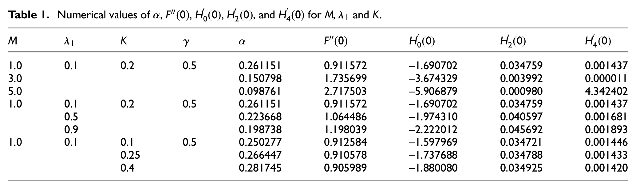
The behavior of physical quantities $C_f$ , $N{u}_x$ and $S{h}_x$ that is influenced by the increasing value of governing parameters, can be observed through the tabular values enlisted in Tables 1, 4 and 5. The numerical values of $F″(0)$ and $\mathbb{A}$ are displayed in Table 1. $\mathbb{A}$ decreases for the increasing $M$ and ${\lambda }_1$ while it increases for increasing $K$ . The numerically computed values of $H_0^{\prime }(0)$ , $H_2^{\prime }(0)$ and $H_4^{\prime }(0)$ are enlisted in Table 2 for some fixed values of $\mathbb{B}-\mathbb{A}=-\mathbb{A},0,\mathbb{A}$ . To validate our numerical values a comparison is made for a limiting case with the results reported by Malvandi et al. ³⁴ in Table 3. A good agreement is found with the previously published data.

Table 1.

Numerical values of $\alpha$ , $F″(0)$ , $H_0^{\prime }(0)$ , $H_2^{\prime }(0)$ , and $H_4^{\prime }(0)$ for $M$ , ${\lambda }_1$ and $K$ .

$M$	${\lambda }_1$	$K$	$\gamma$	$\alpha$	$F″(0)$	$H_0^{\prime }(0)$	$H_2^{\prime }(0)$	$H_4^{\prime }(0)$
1.0	0.1	0.2	0.5	0.261151	0.911572	−1.690702	0.034759	0.001437
3.0				0.150798	1.735699	−3.674329	0.003992	0.000011
5.0				0.098761	2.717503	−5.906879	0.000980	4.342402
1.0	0.1	0.2	0.5	0.261151	0.911572	−1.690702	0.034759	0.001437
	0.5			0.223668	1.064486	−1.974310	0.040597	0.001681
	0.9			0.198738	1.198039	−2.222012	0.045692	0.001893
1.0	0.1	0.1	0.5	0.250277	0.912584	−1.597969	0.034721	0.001446
		0.25		0.266447	0.910578	−1.737688	0.034788	0.001433
		0.4		0.281745	0.905989	−1.880080	0.034925	0.001420

Table 2.

Numerical values of $\mathbb{B}-\mathbb{A}$ and $G_0^{\prime }(0)$ for $M$ , ${\lambda }_1$ , and $K$ .

$M$	${\lambda }_1$	$K$	$\gamma$	$\mathbb{B}-\mathbb{A}$	$G_0^{\prime }(0)$
1.0	0.1	0.2	0.5	−0.261151	1.007541
				0	0.561360
				0.261151	0.115181
3.0	0.1	0.2	0.5	−0.150798	1.302075
				0	0.763295
				0.150798	0.224515
5.0	0.1	0.2	0.5	−0.098761	1.317502
				0	0.757434
				0.098761	0.197366
1.0	0.1	0.2	0.5	−0.261151	1.007541
				0	0.561360
				0.261151	0.115181
1.0	0.5	0.2	0.5	−0.223668	1.048176
				0	0.598303
				0.223668	0.148430
1.0	0.9	0.2	0.5	−0.198738	1.074272
				0	0.622349
				0.198738	0.170426
1.0	0.1	0.1	0.5	−0.250277	0.970416
				0	0.554411
				0.250277	0.138407
1.0	0.1	0.25	0.5	−0.266447	1.027773
				0	0.566328
				0.266447	0.104869
1.0	0.1	0.4	0.5	−0.281745	1.092974
				0	0.585306
				0.281745	0.077641

Table 3.

Comparison for the variation in $\mathbb{B}-\mathbb{A}$ and $G_0^{\prime }(0)$ when $K=0$ with the results reported by Malvandi et al. ³⁴

$M$	$\mathbb{B}-\mathbb{A}$	$G_0^{\prime }(0)$
		Malvandi et al. 34	$\mathrm{Present}$
0.0	−0.647901	1.4065	1.406716
	0	0.6080	0.607959
	0.647901	−0.1906	−0.190636
1.0	−0.541007	1.4240	1.423991
	0	0.5663	0.566316
	0.541007	−0.2913	−0.291359
2.0	−0.393589	1.4541	1.454064
	0	0.5304	0.530443
	0.393589	−0.3932	−0.393177
5.0	−0.190729	1.4880	1.488170
	0	0.5063	0.506304
	0.190729	−0.4754	−0.475561
10.0	−0.098774	1.4970	1.496768
	0	0.5016	0.501646
	0.098774	−0.4937	−0.493476

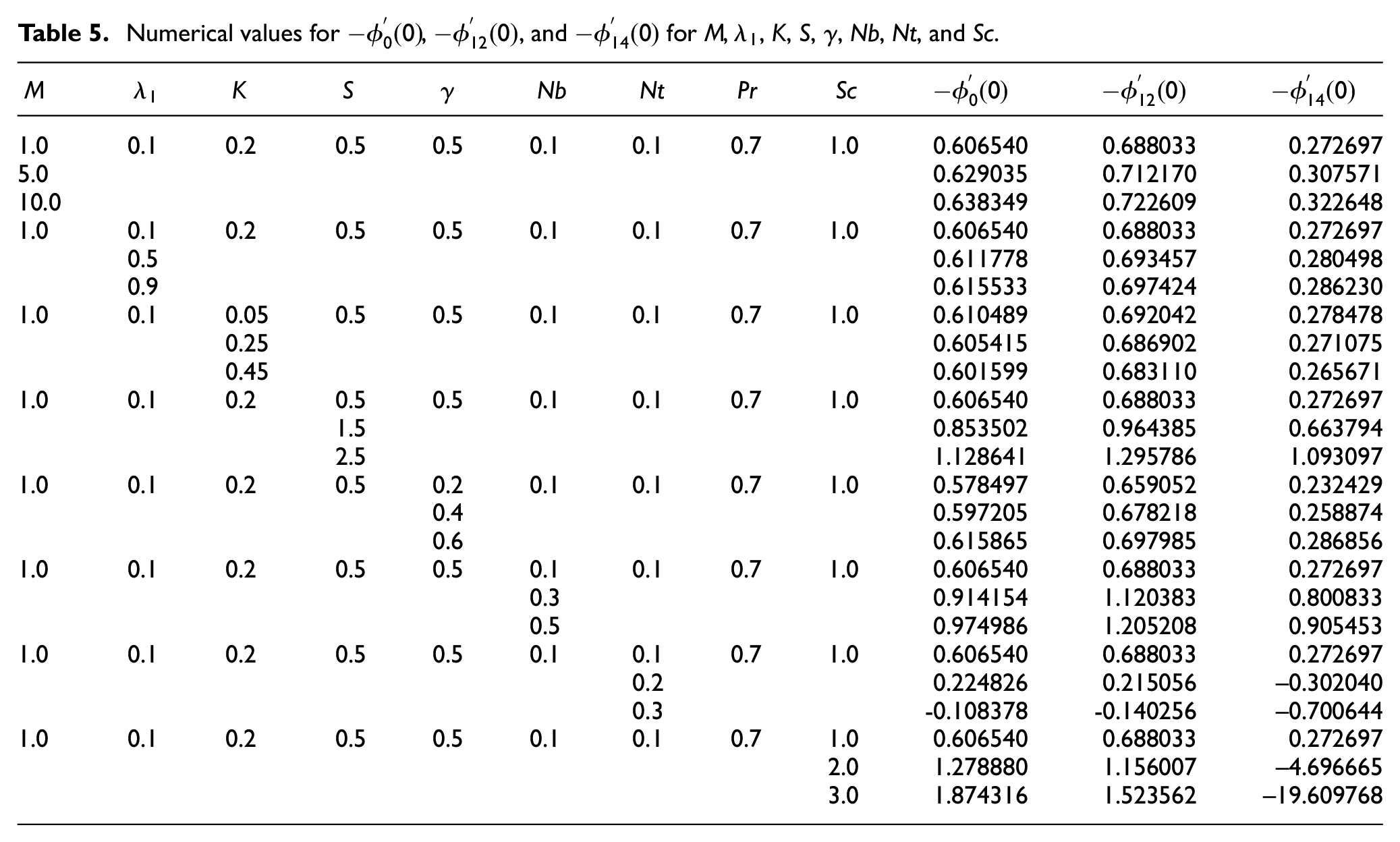
The behavior of skin friction coefficient $C_f$ can be determined with the help of tabulated values of $F″(0)$ in Table 1. An increment in $C_f$ is shown for the increasing $M$ and ${\lambda }_1$ while a reduction in $C_f$ is shown for increasing $K$ . The behavior of $N{u}_x$ can be seen through Table 4. The evaluated results reveal that $N{u}_x$ shows an increment for gradually increasing $M$ , ${\lambda }_1$ , $S$ , $\gamma$ , and $\mathrm{Pr}$ . However, it shows reduction for growing values of $K$ , $\mathrm{Nb}$ and $\mathrm{Nt}$ . Table 5 reports the increment and reduction in $S{h}_x$ . $S{h}_x$ increases for gradually growing parameters $M$ , ${\lambda }_1$ , $S$ , $\gamma$ , $\mathrm{Nb}$ , and $\mathrm{Sc}$ but it decreases for increment in parameters $K$ and $\mathrm{Nt}$ .

Table 4.

Numerical values of $-{\theta }_0^{\prime }(0)$ , $-{\theta }_{12}^{\prime }(0)$ , and $-{\theta }_{14}^{\prime }(0)$ for $M$ , ${\lambda }_1$ , $K$ , $S$ , $\gamma$ , $\mathrm{Nb}$ , $\mathrm{Nt}$ , and $\mathrm{Pr}$ .

$M$	${\lambda }_1$	$K$	$S$	$\gamma$	$\mathrm{Nb}$	$\mathrm{Nt}$	$\mathrm{Pr}$	$\mathrm{Sc}$	$-{\theta }_0^{\prime }(0)$	$-{\theta }_{12}^{\prime }(0)$	$-{\theta }_{14}^{\prime }(0)$
1.0	0.1	0.2	0.5	0.5	0.1	0.1	0.7	1.0	0.766766	1.061854	1.101256
5.0									0.796625	1.082151	1.118731
10.0									0.810641	1.092223	1.127887
1.0	0.1	0.2	0.5	0.5	0.1	0.1	0.7	1.0	0.766766	1.061854	1.101256
	0.5								0.773251	1.066159	1.104823
	0.9								0.778038	1.069359	1.107521
1.0	0.1	0.05	0.5	0.5	0.1	0.1	0.7	1.0	0.771368	1.064852	1.103661
		0.25							0.765459	1.060999	1.100573
		0.45							0.761056	1.058113	1.098278
1.0	0.1	0.2	0.5	0.5	0.1	0.1	0.7	1.0	0.766766	1.061854	1.101256
			1.5						1.271841	1.484864	1.509985
			2.5						1.835775	1.956334	1.971706
1.0	0.1	0.2	0.5	0.2	0.1	0.1	0.7	1.0	0.723744	1.030233	1.072804
				0.4					0.752534	1.051426	1.091863
				0.6					0.780894	1.072177	1.110567
1.0	0.1	0.2	0.5	0.5	0.1	0.1	0.7	1.0	0.766766	1.061854	1.101256
					0.5				0.651222	0.860776	0.940039
					0.9				0.549348	0.693287	0.801936
1.0	0.1	0.2	0.5	0.5	0.1	0.1	0.7	1.0	0.766766	1.061854	1.101256
						0.5			0.655789	0.856601	0.890186
						0.9			0.563820	0.681608	0.666476
1.0	0.1	0.2	0.5	0.5	0.1	0.1	0.3	1.0	0.477691	0.672921	0.687110
							0.5		0.628462	0.880194	0.907291
							0.7		0.766766	1.061854	1.101256

Table 5.

Numerical values for $-{\varphi }_0^{\prime }(0)$ , $-{\varphi }_{12}^{\prime }(0)$ , and $-{\varphi }_{14}^{\prime }(0)$ for $M$ , ${\lambda }_1$ , $K$ , $S$ , $\gamma$ , $\mathrm{Nb}$ , $\mathrm{Nt}$ , and $\mathrm{Sc}$ .

$M$	${\lambda }_1$	$K$	$S$	$\gamma$	$\mathrm{Nb}$	$\mathrm{Nt}$	$\mathrm{Pr}$	$\mathrm{Sc}$	$-{\varphi }_0^{\prime }(0)$	$-{\varphi }_{12}^{\prime }(0)$	$-{\varphi }_{14}^{\prime }(0)$
1.0	0.1	0.2	0.5	0.5	0.1	0.1	0.7	1.0	0.606540	0.688033	0.272697
5.0									0.629035	0.712170	0.307571
10.0									0.638349	0.722609	0.322648
1.0	0.1	0.2	0.5	0.5	0.1	0.1	0.7	1.0	0.606540	0.688033	0.272697
	0.5								0.611778	0.693457	0.280498
	0.9								0.615533	0.697424	0.286230
1.0	0.1	0.05	0.5	0.5	0.1	0.1	0.7	1.0	0.610489	0.692042	0.278478
		0.25							0.605415	0.686902	0.271075
		0.45							0.601599	0.683110	0.265671
1.0	0.1	0.2	0.5	0.5	0.1	0.1	0.7	1.0	0.606540	0.688033	0.272697
			1.5						0.853502	0.964385	0.663794
			2.5						1.128641	1.295786	1.093097
1.0	0.1	0.2	0.5	0.2	0.1	0.1	0.7	1.0	0.578497	0.659052	0.232429
				0.4					0.597205	0.678218	0.258874
				0.6					0.615865	0.697985	0.286856
1.0	0.1	0.2	0.5	0.5	0.1	0.1	0.7	1.0	0.606540	0.688033	0.272697
					0.3				0.914154	1.120383	0.800833
					0.5				0.974986	1.205208	0.905453
1.0	0.1	0.2	0.5	0.5	0.1	0.1	0.7	1.0	0.606540	0.688033	0.272697
						0.2			0.224826	0.215056	−0.302040
						0.3			−0.108378	−0.140256	−0.700644
1.0	0.1	0.2	0.5	0.5	0.1	0.1	0.7	1.0	0.606540	0.688033	0.272697
								2.0	1.278880	1.156007	−4.696665
								3.0	1.874316	1.523562	−19.609768

Conclusion

The numerical investigation of the mathematical problem of two-dimensional oblique stagnation point flow with the MHD effects of incompressible unsteady Jeffrey fluid induced by an oscillatory and stretching sheet has been presented in this article. The numerical solutions of this problem are evaluated with the help of problem-solver BVP MAPLE. The variations in velocity, concentration, and temperature profiles influenced by the governing physical parameters are depicted in graphs. The numerical values are also displayed in tables for the investigation of physical quantities Nusselt number, skin friction coefficient, and Sherwood number. The results are summarized as follows:

• The increasing behavior of $F\prime (y)$ is detected for increasing $M$ , ${\lambda }_1$ , and $S$ with fixed $\gamma <1$ . $K$ with fixed $\gamma <1$ tends to decrease $F\prime (y)$ profile. The results are opposite when $\gamma >1$ .

• Velocity profile $G_0(y)$ behaves as an increasing function of growing $M$ , ${\lambda }_1$ , and $S$ with fixed $\mathbb{B}<0$ and behaves as a decreasing function for growing $K$ with $\mathbb{B}<0$ . The results are the opposite in the case of $\mathbb{B}>0$ .

• $\theta (y)$ and $\varphi (y)$ profiles decrease with growing $M$ for $\gamma >1$ case.

• $S$ , $\gamma$ , and $\mathrm{Pr}$ cause to decrease $\theta (y)$ while $\mathrm{Nb}$ and $\mathrm{Nt}$ cause to increase it for both cases of $\gamma$ .

• $\varphi (y)$ profile shows decreasing the behavior to increasing $\mathrm{Sc}$ , $\mathrm{Nb}$ , and $S$ for both cases of $\gamma$ .

• Skin friction coefficient boosts up with higher values of $M$ and ${\lambda }_1$ while reverse results are shown for increasing $K$ .

• Nusselt number enhances for gradually growing values of $M$ , ${\lambda }_1$ , $S$ , $\gamma$ , and $\mathrm{Pr}$ , and reduces for increasing $\mathrm{Nt}$ , $K$ , and $\mathrm{Nb}$ .

• Sherwood number rises for gradually increasing $M$ , ${\lambda }_1$ , $S$ , $\mathrm{Nb}$ , $\gamma$ , and $\mathrm{Sc}$ . However, it reduces for growing $K$ and $\mathrm{Nt}$ .