Magnetohydrodynamics flow of nanofluid due to stretching/shrinking surface with slip effect

Abstract

This research concerns with the flow of nanofluid due to a stretching/shrinking surface. The underlying problem governs the boundary layer equations for two-dimensional viscous and incompressible fluids in Cartesian coordinate system. The implication of similarity transformations to highly nonlinear partial differential equations renders a system of coupled nonlinear ordinary differential equations. The corresponding system of coupled nonlinear ordinary differential equations is then solved numerically by shooting method. The problem is discussed and investigated graphically subject to different physical parameters of interest.

Introduction

Nanofluids are potential heat transfer fluids with improved thermophysical properties. Generally, such fluids consist of nanometer-sized particles called nanoparticles. These fluids are engineered colloidal suspensions of nanoparticles in a base fluid. The nanoparticles are used in nanofluids which is made of metals, oxides, carbides, or carbon nanotubes. ¹ Choi ¹ commended that thermal conductivity and convective heat transfer of nanoparticles is considerably increased proportional to heat transfer. The enhancement of heat transfer is created by increasing the heat flow process. The investigation based on nanofluids attracted many researcher and scientists all over the world. These fluids are diversified in the area of engineering and industries, which may include nuclear systems cooling, high-power lasers, microwave tubes, solar water heating, engine transmission oil, and biomedical applications.^1,2

The study of such fluids flow over a stretching sheet has gained admirable attention due to its extensive use in engineering applications, such as bundle wrapping, hot rolling, wire rolling, and glass fiber. The study of nanofluids over stretching sheet due to its industrial importance and applications is substantial. Moreover, boundary layer flow and heat transfer over exponentially stretching surface has extensively been investigated because of its application in industry and manufacturing processes, whereas Liu ³ studied boundary layer flow of Newtonian and non-Newtonian fluids over linear and nonlinear stretching surfaces.^4–8 Similar related flow problems with different physical configurations have been reported by many researchers in the previous studies.^9–11

While investigating the flow behavior of nanofluid in different channels, certain physical properties are necessarily discussed. For example, thermal conductivity is the most significant thermophysical property of nanofluids which must be studied to demonstrate the capability of these new engineered suspensions for heat transfer applications. Higher thermal conductivity is desired for effective nanofluids for heat transfer applications. It is worth mentioning that higher values of thermal conductivity are preferred for the operative role of nanofluid in heat transfer applications. In this way, thermal conductivity enables to reduce friction coefficients, to have smaller and higher cooling systems with higher cooling rates, to reduce production of heat transform as well as pumping power, and so on. These characteristics make nanofluids promising for applications like lubricants, hydraulic fluids, coolants, and metal-cutting fluids. ¹² Furthermore, having practical applications in the theory of boundary layer control and thermal protection in high energy flow, the consideration of these fluids becomes significant, referred for instance to the studies of Bidin and Nazar, ¹³ Khanafer et al. ¹⁴ and Makinde and Aziz. ¹⁵ Later, M Turkyilmazoglu ¹⁶ studied relationship between flow due to stretching/shrinking surfaces and heat in two to three dimensions. Also, stagnation point of Jeffrey fluid flow over deformable surfaces has been investigated by M Turkyilmazoglu ¹⁷ by considering magnetic field and slip effects. In addition, the analysis of magnetohydrodynamics (MHD) flow and heat transfer over a stretching/shrinking sheet has a wide range of applications in sheet extrusion in order to make flat plastic sheets. An improved form of final product is achieved by investigating cooling and heat transfer. In recent developments, the flow kinematics has been transformed to yield a slower rate of solidification as compared with conventional fluids such as water and air. Therefore, the idea of introducing magnetic field is appeared to be most attractive while controlling the flow kinematics. Several authors have measured various aspects of problems involving MHD flow effects over stretching sheets in nanofluids, to name a few.^18–21 Following the background, we analyzed MHD flow of nanofluid with slip effects. To the best of authors’ knowledge, the underlying model subject to specified conditions has never been examined. Thus, we aim to provide a numerical solution to the underlying flow problem thereby comparing the results with the existing literature as a special case.

This article is articulated in the following order. The problem is formulated in section “Problem formulation,” whereas non-dimensionalizing is performed using similarity transforms in section “Similarity transformations.” The results are presented in section “Results and discussion” using shooting method and bvp4c MATLAB code. Section “Results and discussion” also includes graphical behavior of flow subject to different physical parameters of interest. Toward the end, problem is concluded in section “Conclusion.”

Problem formulation

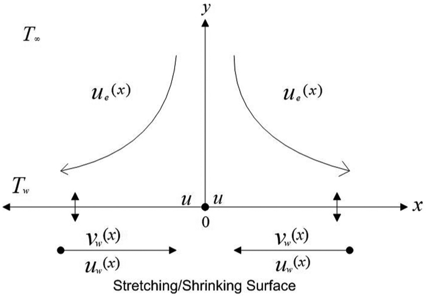
The steady incompressible viscous flow of nanofluid over stretching/shrinking sheet in two dimensions is considered. It is also assumed that sheet is stretching or shrinking along x-axis and constant magnetic field is applied along y-axis which is in perpendicular direction to fluid flow. Moreover, the stretching/shrinking sheet has velocity $u_w(x)$ which varies in the x-direction and temperature $T_w(x)$ is also assumed variable. The flow configuration is shown in Figure 1.

Figure 1.

Flow configuration.

The governing equations for the underlying stagnation point flow model are given as

$$\frac{\partial u}{\partial x}+\frac{\partial v}{\partial y}=0$$

(1)

$$u\frac{\partial u}{\partial x}+v\frac{\partial v}{\partial y}=u_e\frac{d{u}_e}{dx}+\upsilon \frac{{\partial }^{2}u}{\partial y^2}-\frac{\sigma B_o^2}{\rho }(u-u_e)$$

(2)

$$u\frac{\partial T}{\partial x}+v\frac{\partial T}{\partial y}=\alpha \frac{{\partial }^{2}T}{\partial y^2}+\frac{{(\rho c)}_p}{{(\rho c)}_f}\left[D_B\frac{\partial C}{\partial y}\frac{\partial T}{\partial y}+\frac{D_T}{T_{\infty }}{\left(\frac{\partial T}{\partial y}\right)}^2\right]$$

(3)

$$u\frac{\partial C}{\partial x}+v\frac{\partial C}{\partial y}=D_B\frac{{\partial }^{2}C}{\partial y^2}+\frac{D_T}{T_{\infty }}\left(\frac{{\partial }^{2}T}{\partial y^2}\right)$$

(4)

whereas the associated boundary conditions are

$$\begin{array}{l}v=v_w(x),u=u_w(x)+M(x)\mu \frac{\partial u}{\partial y},\\ T=T_w(x)+N(x)\mu \frac{\partial T}{\partial y}\\ C=C_w(x)+N_1(x)\mu \frac{\partial C}{\partial y}\mathrm{at}y=0\\ u\to u_e(x),T\to T_{\infty },C\to C_{\infty }\mathrm{as}y\to \infty \end{array}$$

(5)

Here, u and v are longitudinal and transverse components of velocity, respectively, $u_e$ is external velocity of fluid, $\upsilon$ is kinematic viscosity, $\sigma$ represents electric conductivity, $B_0$ stands for constant magnetic field, $\rho$ is the density of fluid, T is temperature, $\alpha$ denotes the thermal diffusivity, $(\rho c{)}_p$ represents the effective heat capacity of nanoparticles, $(\rho c{)}_f$ denotes the heat capacity of fluid, $D_B$ represents the Brownian diffusivity, $D_T$ denotes the thermophoretic diffusion coefficient, C stands for concentration, and $T_{\infty }$ is ambient temperature of fluid. Furthermore, $M(x)$ , $N(x)$ , $N_1(x)$ , $v_w(x)$ , $u_e(x)$ , and $u_w(x)$ are defined as

$$\begin{array}{l}{u}_e\left(x\right)=a{x}^m,u_w\left(x\right)=c{x}^m,T_w\left(x\right)=T_{\infty }+T_0{x}^n\\ N_1(x)=\sqrt{\frac{2}{a\upsilon (m+1)}}{x}^{\frac{1-m}{2}}\frac{B_1}{\rho },v_w(x)=-\sqrt{\frac{a(m+1)\upsilon }{2}}{x}^{\frac{m-1}{2}}S\\ N(x)=\sqrt{\frac{2}{a\upsilon (m+1)}}{x}^{\frac{1-m}{2}}\frac{B}{\rho },M(x)=\sqrt{\frac{2}{a\upsilon (m+1)}}{x}^{\frac{1-m}{2}}\frac{A}{\rho }\end{array}$$

(6)

where $a,c$ , and m are the positive constants. Likewise, $M(x)$ , $N(x)$ , and $N_1(x)$ are representing the velocity, temperature, and concentration slip parameters; $\mu$ is dynamic viscosity; $C_w$ denotes concentration of a fluid at wall; and $C_{\infty }$ denotes the ambient concentration of a fluid. It is worthwhile to mention that the model problem equations (1)–(5) are the modified nature of the study of Fauzi et al. ⁸ including the additional effects of MHD nanofluid subject to slip boundary condition.

Similarity transformations

The following similarity transformations are used to solve the governing equations (1)–(4)

$$\begin{array}{l}\eta =y{x}^{\frac{(m-1)}{2}}\sqrt{\frac{a(m+1)}{2\upsilon }},\theta (\eta )=\frac{T-T_{\infty }}{T_w-T_{\infty }},\\ \phi (\eta )=\frac{C-C_{\infty }}{C_w-C_{\infty }},\psi =\sqrt{\frac{2\upsilon a}{m+1}}{x}^{\frac{m+1}{2}}f(\eta )\end{array}$$

(7)

where the stream function $\psi$ is defined in terms of longitudinal $(u)$ and transverse $(v)$ components of velocity

$$u=\frac{\partial \psi }{\partial y},v=-\frac{\partial \psi }{\partial x}$$

Thus, we have

$$\begin{array}{l}u=a{x}^m{f}^{\prime }(\eta ),\\ v=-\sqrt{\frac{a(m+1)\upsilon }{2}}{x}^{\frac{(m-1)}{2}}\left[f(\eta )+\frac{m-1}{m+1}\eta f^{\prime }(\eta )\right]\end{array}$$

(8)

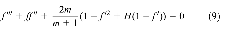
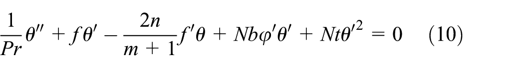
The equation of continuity (1) is satisfied identically using equations (7) and (8). In view of above, equations (2)–(5) take the form

$$f^{‴}+f{f}^{″}+\frac{2m}{m+1}(1-{f^{\prime }}^2+H(1-f^{\prime }))=0$$

(9)

$$\frac{1}{Pr}{\theta }^{″}+f{\theta }^{\prime }-\frac{2n}{m+1}{f}^{\prime }\theta +Nb{\phi }^{\prime }{\theta }^{\prime }+Nt{\theta \prime }^2=0$$

(10)

$${\phi }^{″}+PrLe\left(f{\phi }^{\prime }-\frac{2n}{m+1}{f}^{\prime }\phi \right)+\frac{Nt}{Nb}{\theta }^{″}=0$$

(11)

and associated boundary conditions are

$$\begin{array}{l}f(0)=S,f^{\prime }(0)=\lambda +\mathrm{A}{f}^{″}(0),\theta (0)=1+B{\theta }^{\prime }(0),\\ \phi (0)=1+B_1{\phi }^{\prime }(0)\mathrm{when}\eta =0\\ f^{\prime }(\infty )=1,\theta (\infty )=0,\phi (\infty )=0\mathrm{as}\eta \to \infty \end{array}$$

(12)

where prime denotes differentiation with respect to $\eta$ and $H=\sigma /a\rho m$ is magnetic parameter, Pr is Prandtl number, $\mathrm{Nt}(\mathrm{Nt}=D_B((\rho {)}_{\mathrm{cp}}/(\rho {)}_{\mathrm{cf}})((C_w-C_{\infty })/\upsilon ))$ stands for thermophoresis parameter, $\mathrm{Nb}(N_b=(D_T/T_{\infty })((\rho {)}_{\mathrm{cp}}/(\rho {)}_{\mathrm{cf}})((T_w-T_{\infty })/\upsilon ))$ represents Brownian motion parameter, and Le denotes the Lewis number. Additionally, S stands for constant mass flux parameter which is greater than zero in suction $(S>0)$ and less than zero in the case of injection $(S<0)$ . Moreover, $A,B$ , and $B_1$ are the positive constant slip parameters, and $\lambda =c/a$ represents the stretching/shrinking parameter; if $c<0$ implies $\lambda <0$ , then sheet will be shrinking, otherwise it is stretching.

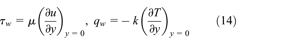
The physical parameters skin friction coefficient, local Nusselt number, and Sherwood number are defined as

$$\begin{array}{l}{C}_f=\frac{{\tau }_w}{\rho {u_e}^2},N{u}_x=\frac{x{q}_w}{k(T_w-T_{\infty })},\\ S{h}_x=\frac{-x}{C_w-C_{\infty }}{\left(\frac{\partial C}{\partial y}\right)}_{y=0}\end{array}$$

(13)

where

$${\tau }_w=\mu {\left(\frac{\partial u}{\partial y}\right)}_{y=0},q_w=-k{\left(\frac{\partial T}{\partial y}\right)}_{y=0}$$

(14)

with $C_f$ meaning skin friction coefficient, local Nusselt number denoted by $N{u}_x$ , $S{h}_x$ stands for Sherwood number, ${\tau }_w$ is shear stress over a surface of sheet, $q_w$ is characterized by heat flux of the stretching or shrinking sheet, and k is a thermal conductivity of the fluid. The correct range of values of dimensionless physical parameters involved in the governing equations can been seen in the article by M Turkyilmazoglu. ¹⁶ Again using equations (7) and (8) in equation (14) and then substituting equation (14) into equation (13), we obtain the following expressions

$$\begin{array}{l}{{\mathrm{Re}}_x}^{\frac{1}{2}}{C}_f=\sqrt{\frac{m+1}{2}}{f}^{″}(0),{{\mathrm{Re}}_x}^{-\frac{1}{2}}N{u}_x=-\sqrt{\frac{m+1}{2}}{\theta }^{\prime }(0),\\ {{\mathrm{Re}}_x}^{-\frac{1}{2}}S{h}_x=-\sqrt{\frac{m+1}{2}}{\varphi }^{\prime }(0)\end{array}$$

(15)

Here, ${\mathrm{Re}}_x=u_e(x)x/\upsilon$ is the local Reynolds number.

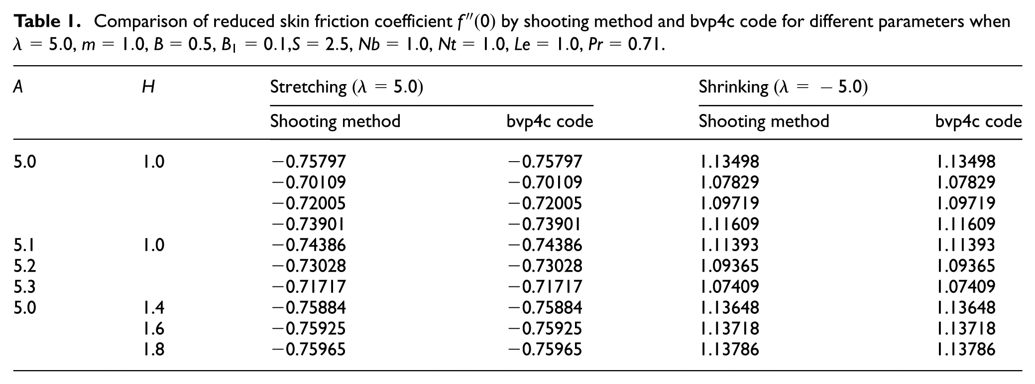
It is evident through equations (9)–(11) along with boundary conditions equation (12) that the exact analytical solution is not conceivable. For the reason, we are only left with the use of some numerical treatment for the system of equation. The shooting method is preferred to obtain approximate solution which is then compared with bvp4c MATLAB code. The results will be validated while computing the physical parameters such as reduced skin coefficient friction, reduced Nusselt number, and reduced Sherwood number for both the stretching and shrinking cases. The comparative analysis is then provided through Tables 1–3.

Table 1.

Comparison of reduced skin friction coefficient $f″(0)$ by shooting method and bvp4c code for different parameters when $\lambda =5.0$ , $m=1.0$ , $B=0.5$ , $B_1=0.1$ , $S=2.5$ , $\mathrm{Nb}=1.0$ , $\mathrm{Nt}=1.0$ , $\mathrm{Le}=1.0$ , $\mathrm{Pr}=0.71$ .

A	H	Stretching $(\lambda =5.0)$		Shrinking $(\lambda =-5.0)$
		Shooting method	bvp4c code	Shooting method	bvp4c code
5.0	1.0	−0.75797	−0.75797	1.13498	1.13498
		−0.70109	−0.70109	1.07829	1.07829
		−0.72005	−0.72005	1.09719	1.09719
		−0.73901	−0.73901	1.11609	1.11609
5.1	1.0	−0.74386	−0.74386	1.11393	1.11393
5.2		−0.73028	−0.73028	1.09365	1.09365
5.3		−0.71717	−0.71717	1.07409	1.07409
5.0	1.4	−0.75884	−0.75884	1.13648	1.13648
	1.6	−0.75925	−0.75925	1.13718	1.13718
	1.8	−0.75965	−0.75965	1.13786	1.13786

Table 2.

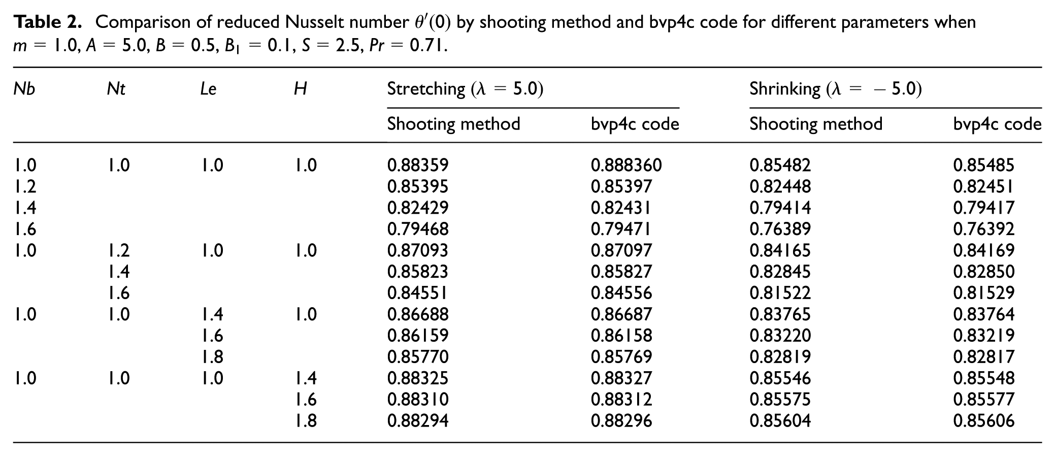
Comparison of reduced Nusselt number $\theta \prime (0)$ by shooting method and bvp4c code for different parameters when $m=1.0$ , $A=5.0$ , $B=0.5$ , $B_1=0.1$ , $S=2.5$ , $\mathrm{Pr}=0.71$ .

Nb	Nt	Le	H	Stretching $(\lambda =5.0)$		Shrinking $(\lambda =-5.0)$
				Shooting method	bvp4c code	Shooting method	bvp4c code
1.0	1.0	1.0	1.0	0.88359	0.888360	0.85482	0.85485
1.2				0.85395	0.85397	0.82448	0.82451
1.4				0.82429	0.82431	0.79414	0.79417
1.6				0.79468	0.79471	0.76389	0.76392
1.0	1.2	1.0	1.0	0.87093	0.87097	0.84165	0.84169
	1.4			0.85823	0.85827	0.82845	0.82850
	1.6			0.84551	0.84556	0.81522	0.81529
1.0	1.0	1.4	1.0	0.86688	0.86687	0.83765	0.83764
		1.6		0.86159	0.86158	0.83220	0.83219
		1.8		0.85770	0.85769	0.82819	0.82817
1.0	1.0	1.0	1.4	0.88325	0.88327	0.85546	0.85548
			1.6	0.88310	0.88312	0.85575	0.85577
			1.8	0.88294	0.88296	0.85604	0.85606

Table 3.

Comparison of reduced Sherwood number $\phi \prime (0)$ by shooting method and bvp4c code for different parameters when $m=1.0$ , $A=5.0$ , $B=0.5$ , $B_1=0.1$ , $S=2.5$ , $\mathrm{Pr}=0.71$ .

Nb	Nt	Le	H	Stretching $(\lambda =5.0)$		Shrinking $(\lambda =-5.0)$
				Shooting method	bvp4c code	Shooting method	bvp4c code
1.0	1.0	1.0	1.0	1.39111	1.39065	1.33521	1.33462
1.2				1.50170	1.50129	1.44437	1.44383
1.4				1.58066	1.58028	1.52229	1.52180
1.6				1.63981	1.63945	1.58064	1.58017
1.0	1.2	1.0	1.0	1.29943	1.29885	1.24710	1.24635
	1.4			1.21229	1.21158	1.16381	1.16288
	1.6			1.12967	1.12881	1.08530	1.08418
1.0	1.0	1.4	1.0	1.91542	1.91529	184773	1.84754
		1.6		2.14830	2.14820	2.07681	2.07667
		1.8		2.36543	2.36535	2.29116	2.29105
1.0	1.0	1.0	1.4	1.39036	1.38990	1.33654	1.33595
			1.6	1.39001	1.38955	1.33716	1.33657
			1.8	1.389669	1.38921	1.33775	1.33716

Results and discussion

This section provides significant tabular and graphical illustration to demonstrate velocity, temperature, and concentration profiles against similarity parameter $\eta$ for both stretching and shrinking cases. We also compare reduced skin coefficient friction $f″(0)$ , reduced local Nusselt number $\theta \prime (0)$ , and reduced Sherwood number $\phi \prime (0)$ for various values of parameters through shooting method and bvp4c code. Tables 1–3 are provided to visualize effects of reduced skin coefficient friction $f″(0)$ , reduced local Nusselt number $\theta \prime (0)$ , and reduced Sherwood number $\phi \prime (0)$ on various physical parameters of interest. The behavior of reduced skin coefficient friction $f″(0)$ is discussed in Table 1 for both stretching and shrinking cases. It is noticed that reduced skin coefficient has lesser effects on higher values of stretching/shrinking parameter $\lambda$ and magnetic parameter H, but it has stronger effects on increasing values of velocity slip parameter A for stretching case. However, for shrinking case, reduced skin coefficient friction $f″(0)$ exhibits opposite effects to stretching case. The effects of reduced local Nusselt number $\theta \prime (0)$ on several parameters are observed through Table 2 for stretching and shrinking cases, respectively. It is seen that higher values of Brownian motion parameter Nb, thermophoresis parameter Nt, and Lewis number Le produce minimal effects for reduced local Nusselt number $\theta \prime (0)$ for both cases, whereas magnetic effects are negligible on reduced local Nusselt number $\theta \prime (0)$ for stretching as well as shrinking case. Similarly, Table 3 describes the behavior of reduced Sherwood number $\phi \prime (0)$ on different parameters. It is observed that an increment in Brownian motion parameter Nb and Lewis number Le achieve the stronger effects for reduced Sherwood number $\phi \prime (0)$ , whereas it has minimal effects on higher values of thermophoresis parameter Nt for both cases. And again, magnetic effects are negligible on reduced Sherwood number $\phi \prime (0)$ for stretching case as well as shrinking case.

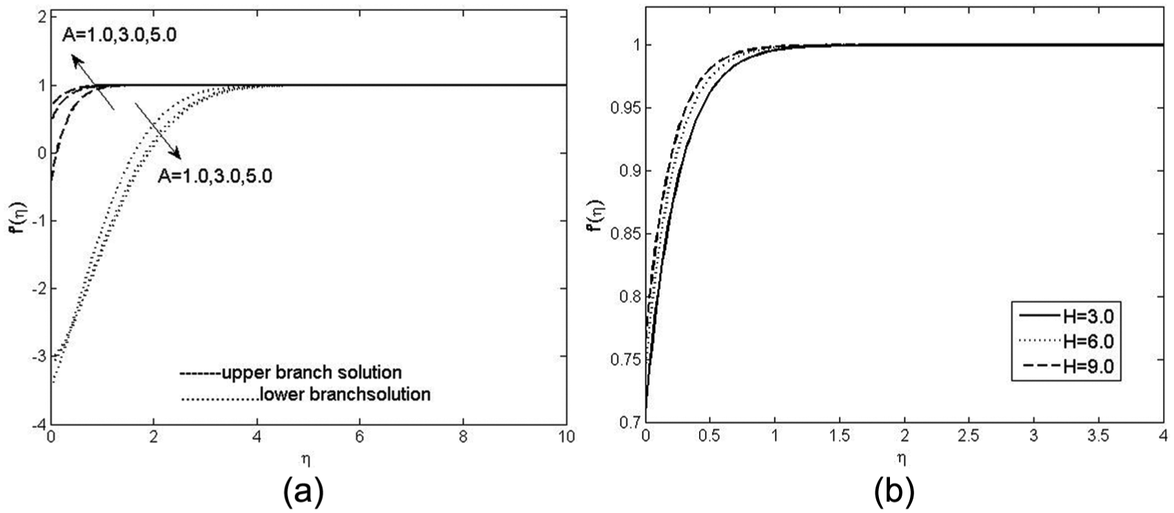
As mentioned earlier, the set of equations (9)–(12) is solved numerically with the help of shooting method. Figures 2–9 are illustrated to discuss velocity, temperature, and concentration profiles for both stretching and shrinking sheets. In continuation, Figure 2(a) and (b) is plotted for velocity profile $f\prime (\eta )$ versus $\eta$ in case of stretching sheet. It is depicted that the velocity profile $f\prime (\eta )$ decreases by increasing the velocity slip parameter A and magnetic parameter H, whereas we obtain dual solution for velocity slip parameter A in case of shrinking sheet (see Figure 6). It is noticed that the upper branch solution increases the velocity profile, whereas lower branch solution decreases the velocity profile $f\prime (\eta )$ by increasing the velocity slip parameter A. Also, the velocity profile $f\prime (\eta )$ obtained higher values on increasing the magnetic parameter H as shown in Figure 6. However, the temperature profile $\theta (\eta )$ and concentration profile $\phi (\eta )$ remain invariant due to magnetic effects in either case.

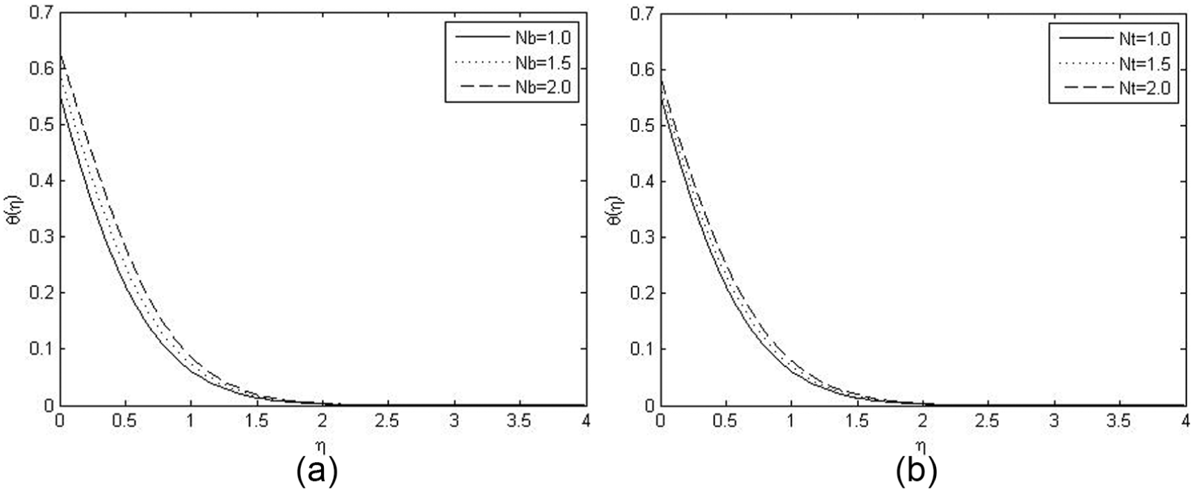
In addition, Figures 3 and 7 are illustrated for temperature profile $\theta (\eta )$ against different values of parameter of interest. We observe that temperature profile $\theta (\eta )$ is decreasing on higher values of thermal slip parameter B in both cases while thermal boundary layer is reduced. Also, it is noticed that temperature profile $\theta (\eta )$ and thermal boundary layer thickness are declining with increasing Prandtl number Pr for both stretching and shrinking sheets. There exists an inverse relation between thermal diffusivity $\alpha$ and Prandtl number Pr; that is, thermal diffusivity $\alpha$ decreases by enhancing values of Prandtl number Pr. Such lowest thermal diffusivity $\alpha$ implies weaker temperature profile $\theta (\eta )$ . But the temperature profile $\theta (\eta )$ has stronger effects on increasing value of Brownian motion parameter Nb and thermophoresis parameter Nt for both stretching and shrinking sheets as given in Figures 4 and 8. It is worth commenting that the thermal boundary layer thickness also increases for such situation.

Moreover, Figures 5 and 9 demonstrate concentration profile $\theta (\eta )$ which measures minimal effects on higher values of concentration slip parameter $B_1$ , Lewis number Le, Brownian motion parameter Nb, and Prandtl number Pr for both stretching and shrinking cases which ultimately decreases the boundary layer thickness. Whereas, an increment in thermophorises parameter Nt achieves stronger concentration profile $\theta (\eta )$ for both sheets (see Figures 5(e) and 9(e)).

Stretching case

Figure 2.

Velocity profile $f\prime (\eta )$ versus $\eta$ by fixing $\lambda =5.0$ , $\mathrm{Pr}=0.71$ $B=0.5$ , $B_1=0.1$ , $\mathrm{Le}=1.0$ , $\mathrm{Nb}=1.0$ , $\mathrm{Nt}=1.0$ , $S=2.5$ : (a) for different values of A and (b) for different values of H.

Figure 3.

Temperature profile $\theta (\eta )$ versus $\eta$ by fixing $\lambda =5.0$ , $H=7.0$ , $A=5.0$ , $B_1=0.1$ , $\mathrm{Le}=1.0$ , $\mathrm{Nb}=1.0$ , $\mathrm{Nt}=1.0$ , $S=2.5$ : (a) for different values of B and (b) for different values of Pr.

Figure 4.

Temperature profile $\theta (\eta )$ versus $\eta$ by fixing $\lambda =5.0$ , $H=7.0$ , $A=5.0$ , $B_1=0.1$ , $\mathrm{Le}=1.0$ , $\mathrm{Pr}=0.71$ , $B=0.5$ , $S=2.5$ : (a) for different values of Nb and (b) for different values of Nt.

Figure 5.

Concentration profile $\phi (\eta )$ versus $\eta$ by fixing $H=7.0$ , $\mathrm{Nt}=1.0$ , $A=5.0$ , $B=0.5$ , $S=2.5$ : (a) for different values of Nt, (b) for different values of Le, (c) for different values of $B_1$ , (d) for different values of Pr, and (e) for different values of $\mathrm{Nt}.$

Figure 6.

Velocity profile $f\prime (\eta )$ versus $\eta$ by fixing $\lambda =-5.0$ for, $\mathrm{Pr}=0.71$ $B=0.5$ , $B_1=0.1$ , $\mathrm{Le}=1.0$ , $\mathrm{Nb}=1.0$ , $\mathrm{Nt}=1.0$ , $S=2.5$ : (a) for different values of A and (b) for different values of H.

Figure 7.

Temperature profile $\theta (\eta )$ versus $\eta$ by fixing $\lambda =-5.0$ , $H=7.0$ , $A=5.0$ , $B_1=0.1$ , $\mathrm{Le}=1.0$ , $\mathrm{Nb}=1.0$ , $\mathrm{Nt}=1.0$ , $S=2.5$ : (a) for different values of B and (b) for different values of $\mathrm{Pr}.$

Figure 8.

Temperature profile $\theta (\eta )$ versus $\eta$ by fixing $\lambda =-5.0$ , $H=7.0$ , $A=5.0$ , $B_1=0.1$ , $\mathrm{Le}=1.0$ , $\mathrm{Pr}=0.71$ , $B=0.5$ , $S=2.5$ : (a) for different values of Nt and (b) for different values of $\mathrm{Nb}.$

Figure 9.

Concentration profile $\phi (\eta )$ versus $\eta$ by fixing $H=7.0$ , $\mathrm{Nt}=1.0$ , $A=5.0$ , $B=0.5$ , $S=2.5$ : (a) for different values of Le, (b) for different values of Pr, (c) for different values of $B_1$ , (d) for different values of Nb, and (e) for different values of $\mathrm{Nt}.$

Shrinking case

Figure 10(a) and (b) shows velocity and temperature profile in the absence of magnetic field and nanofluid. In this setting, the obtained graphs are in close tie with that of the study of Fauzi et al. ⁸ In this way, the obtained solution is validated with existing published data as a special case.

Figure 10.

(a) Velocity profile and (b) temperature profile by fixing $\lambda =-5.0$ , $S=2.5$ , m = n = 1 and B = 0.5.

Conclusion

In this article, we have investigated MHD flow of nanofluid due to stretching/shrinking surface. The use of similarity transforms together with shooting method render solution to the governing problem. The key findings of this article are summarized below:

• Magnetic effects are negligible on temperature profile $\theta (\eta )$ and concentration profile $\phi (\eta )$ in both shrinking and stretching cases.

• Higher values of magnetic parameter H imply stronger velocity profile $f\prime (\eta )$ in shrinking case and weaker velocity profile $f\prime (\eta )$ in stretching case.

• On increasing velocity slip parameter A, velocity profile $f\prime (\eta )$ is decreasing for both stretching and shrinking cases while it is increasing in upper branch solution and decreasing in lower branch solution.

• Higher Prandtl number Pr yields weaker temperature profile $\theta (\eta )$ and concentration profile $\phi (\eta )$ for shrinking case as well as stretching case.

• Likewise, thermal boundary layer thickness and concentration boundary layer thickness are diminishing by raising the values of Prandtl number Pr in both cases.

• An increment in Brownian motion parameter Nb produces a weaker concentration profile $\phi (\eta )$ in shrinking case and stretching case.

• Temperature profile $\theta (\eta )$ and concentration profile $\phi (\eta )$ have similar behavior on thermal slip parameter B, concentration slip parameter $B_1$ , Lewis number Le, Prandtl number Pr, and thermophorises parameter Nt for shrinking case as well as stretching case.