Sage Journals: Discover world-class research

Abstract

Nowadays, multi-fault diagnosis has become the most interesting topic for researchers, since it has lately attracted a substantial attention. The most published works recently have considered defects detection, identification, and classification as the toughest challenge for rotating machinery monitoring. As feature extraction requires robust techniques for online inspection with a high level of expertise to make automatic decisions on the running machine health status, a robust approach is required to adjust the misclassification of the extracted features, especially under various working conditions. In this paper, we propose the combination of two Time Domain Features (TDFs) in tandem with Singular Value Decomposition (SVD) and Fuzzy Logic System (FLS) to build an enhanced fault diagnosis technique for rolling bearing. The original vibration signal is divided first into several data samples. Thereafter, TDFs are applied on each sample to construct a feature matrix during the feature extraction step. Afterwards, SVD is performed on the obtained matrices in order to reduce their dimension and select the most stable vectors (singular values). Finally, FLS is employed as a powerful tool for automatic feature classification. Experimental results confirm that our suggested approach can enhance the ability to assess the degradation of bearing faults with a higher recognition sensitivity even under different working conditions.

Keywords

Faults diagnosis feature extraction feature classification bearing faults time domain features fuzzy logic system

Introduction

As key mechanical parts in rotating machines, bearings are often the heart of a wide range of industrial mechanisms, such as wind turbines and helicopters. However, they are considered as the most vulnerable parts due to their harsh working conditions. A sudden bearing failure may decrease the performance of the entire system and even lead to fatal damages. Therefore, the recent attention to condition-based and predictive maintenance of industrial assets, as well as product safety, have led to a growing focus on bearings condition monitoring. Vibration analysis has been and remains widely used as a predictive maintenance strategy because vibration signals carry a lot of valuable information that gives an insight about the operating machine health condition. When the shaft rotates inside a given machine, both frictional and rotational forces are created. The vibrations produced by these forces are transmitted through the bearings to the gearbox housing. In ordinary working conditions, each specific machine element produces its own relatively stable vibration patterns which are known as the vibration signatures.¹ These signatures are considered as a reference in order to determine any increase in the vibration level that is probably caused by a gear or a bearing failure. The change in the vibration signature can be used to detect emerging faults at an early stage before they become critical. Vibration monitoring techniques use the modified vibration signature to detect, locate, and diagnose the affected part. Vibration analysis is a more powerful tool than other condition monitoring methods like oil analysis, ultrasonic signals, etc, since a small bearing defect increases the amplitude of the acquired vibration signal.¹ However, these signals are often affected by contributions from many different components in addition of the background noise. Therefore, the choice of an appropriate technique becomes crucial and depends significantly on the nature of the captured data. Consequently, many signal processing techniques have been proposed by researchers during decades. The most popular ones include time domain, frequency domain and time–frequency domain as well. Several studies have focused on time domain analysis using pattern recognition basing on statistical characteristics which contribute to describe the machine’s state.² Time domain methods are applied directly on vibration signals in order to detect the change in their amplitude and energy distribution in the present of a bearing failure.³ Frequency or spectrum domain analysis is probably the most common tool used to identify a defective gear.⁴ The vibration signals produced by a machine component are composed of certain frequencies that remain unchanged, although their levels may change. The defective tooth generates a periodic signal with a unique characteristic frequency.⁵ Unlike temporal analysis, frequency analysis identifies the position of the defect by tracking its characteristic frequency. However, spectrum domain analysis cannot handle the non-stationary signals, which are often very frequent in the event of machine part failure. Time-frequency domain methods allow a simultaneous vibration signals analysis in both time and frequency domains. Vibration signals consist of three important elements: “a sinusoidal component due to time varying loading, a broad-band impulsive component due to the fault impact, and random noise.⁶” Time-frequency analysis has been developed for these non-stationary signals. Non-stationary signals are better described by a time-frequency distribution to show the signal’s energy distribution over a two-dimensional space (time and frequency).⁷ Researchers have developed several time-frequency analysis methods to monitor the rotating machine health state. Short-Time Fourier Transform (STFT),^8,9 Wigner Ville Distribution (WVD),^10–12 Wavelet Transform (WT),^13,14 and Hilbert–Huang Transform (HHT)^15,16 are the most commonly used time-frequency techniques and recently Fast Kurtogram^17–19 and Autogram.^20–22 However, time-frequency methods have the ability to detect the occurrence of a bearing failure, but without giving any information about its nature. Moreover, the variation in load and speed of the rotating machine will eventually lead to inaccurate classification results.²³ Currently, intelligent classification techniques are the outstanding methods for bearings condition monitoring.^23–26 Intelligent classification strategies contain two main steps: feature extraction and intelligent classification. The features extraction is the key step part in fault recognition and identification; an accurate features extraction process allows the extraction of the most relevant information from the raw vibration signal. Where, the secret of the accurate classification is directly related to the choice of the most advanced signal processing algorithms. Many researchers have suggested efficient techniques to extract rolling bearing defect features using vibration signals. Zair et al.²⁴ have proposed a combination between Empirical Mode Decomposition (EMD), Principal Component Analysis (PCA) and Fuzzy Entropy as a feature extraction method to identify bearing faults using experimental vibration signals. However, EMD suffers from two disadvantages: mode mixing, in which waves having identical frequencies are assigned to separate IMFs, and the end effect which gives inaccurate instantaneous values on either signal sides.^27,28 To resolve this issue, Zhao et al.²⁹ have proposed a new fault feature extraction approach based on Ensemble EMD (EEMD) and multi-scale fuzzy entropy for bearing condition monitoring. EEMD adds white noise with finite amplitude to the raw signal during the decomposition step. This procedure is repeatedly performed with several white noise sets to obtain the corresponding IMFs ensemble averages reducing by that the chance of the mode mixing.^27,28 Usually, vibration signals are often filled with real background noise which obscures the defect signature and the white noise series will raise the noise amplitude making it even harder to detect the gear failure.³⁰ An alternative decomposition method, Discrete Wavelet Transfer (DWT), has been extensively used in several works and literatures for the feature extraction phase.^31–34 DWT decomposes the vibration signal using a band-pass filter in time and frequency into a series of signals with a specific frequency band. However, the dyadic step in the sub-sampling process appears to be the major limit in DWT. Maximal Overlap Discrete Wavelet Transform (MODWT) came out as an optimized version of DWT to handle the sub-sampling step, yet it still suffers from low frequency resolution as DWT does.²⁶ Maximal Overlap Discrete Wavelet Packet Transform (MODWPT) replaces MODWT and DWT for a better resolution.²⁶ Afia et al.²⁶ developed a new intelligent technique based on MODWPT, entropy for the feature extraction stage and artificial neural network (ANN) to detect and distinguish different types of defects under several loads and speeds. However, MODWPT is not a multi-rate decomposition method, making the feature extraction process very time consuming, which is not recommended for online condition monitoring of industrial devices.²⁰ In machine learning and artificial intelligence, the main purpose remains to find the most relevant features that play a dominant role in determining and influencing output results. Time energy indicators, such as Standard Deviation (SD), entropy (EN), kurtosis (KU), variance (VAR), etc. were used as time domain features (TDFs) through advanced signal processing algorithms to extract the different features matrices.^23,24,26 However, these features matrices have a huge dimension which may lead to serious problems in the classification process and disrupt the most powerful classification algorithms, as well as, it makes the process considerably slow. Bellman,³⁵ named this issue by ‘the curse of dimensionality’ for their harmful influence on the features classification step. Therefore, dimensionality reduction plays a major role in feature classification. A smaller and relevant dimensional size might be helpful in identifying data patterns in feature classification phase. Basically, dimensionality reduction is a mapping from a multidimensional feature space to a reduced dimensions space. Principal component analysis (PCA)^26,36,37 and singular value decomposition (SVD)^38,39 are the most used methods for dimensional reduction. SVD is an excellent matrix analysis technique which has been extensively used for noise reduction, data compression, and feature extraction.^38,39 After feature extraction procedure, feature classification seems to be the second most difficult task. It is a complex procedure which requires a powerful classification tools based on an artificial intelligence. Based on fuzzy set memberships, FLS is a simple classification method which is considered to be one of the most efficient techniques for fault diagnosis that makes a non-autonomous learning by the intervention of an expert.^40,41 FLS is computer software application which simulates the expert’s inference process and performs an expert’s action manner.^40,41 FLS uses fuzzy logic, fuzzy numbers and sets to reflect and handle inaccurate and unclear knowledge.^40,41 Information about the rotating machine condition exhibit some degree of imprecision and uncertainty, that cannot reasonably be solved by traditional expertizing systems like neural networks. Thus, FLS has proven to be more adequate to diagnose defects in rotating equipment’s without depth knowledge and big database.

In this paper, a new intelligent automatic bearing fault diagnosis technique is proposed. Our hybrid technique combines two TDFs (Standard deviation and entropy), SVD and FLS in order to detect and to distinguish between different defects types under several loads and speeds. The paper is organized as follows: section “Introduction” involves an introduction of the work and a brief literature review. Section “Mathematical background” contains mathematical background, and further a straightforwardly experimental procedure. Results and discussion are given in section “Experimental study.” And finally the paper is ended with a conclusion and references.

Mathematical background

Feature extraction based on temporal analysis

In this sub-section, we will discuss the concept of feature extraction for assessing bearing performance degradations. Statistical features provide a valuable tool that discovers the change in vibration signal amplitude and energy distribution due to the event of a bearing failure.

In order to extract the defect information from the bearing time data, time energy indicators such as standard deviation (SD), entropy (EN), variance (VAR) and kurtosis (KU) are presented in equations (1) to (4), respectively⁴²:

X_{Std} = \sqrt{\frac{1}{N - 1} \sum_{j = 1}^{N} {(x_{j} - X_{mean})}^{2}}

(1)

X_{Ig - entropy} = \sum_{i} \log (x_{i}^{2})

(2)

X_{kur} = \frac{1}{X_{rms}^{4}} \sum_{i = 1}^{N} {(x_{i} - X_{mean})}^{4}

(3)

X_{var} = \frac{n \sum x^{2} - (\sum x)^{2}}{n (n - 1)}

(4)

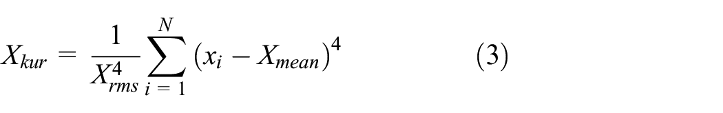
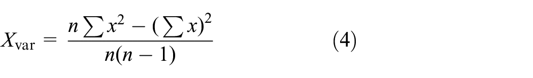
Where i is the sample of signal x, N represents the length.

In our approach, the original vibration data is first divided using equation (5) into many slices, whereby the time of each slice is greater than the bearing defect frequency period to avoid any loss of relevant information. Afterwards, SD and EN indicators are applied to every signal sample in order to calculate the feature matrices.

T_{sample} (s) = \frac{N_{t}}{N_{i}} • {f^{- 1}}_{sampling}

(5)

Where; N_t is the total signal length, f_s is the sampling frequency while N_i is the number of slices.

Singular value decomposition

Singular value decomposition (SVD) is an excellent matrix analysis technique which has been extensively used for noise reduction, data compression and feature extraction. The singular value decomposition is a matrix transformation algorithm that decomposes any given matrix M(m×n) into three matrices U, Σ and V as follows^38,39:

M = U Σ V^{T}

(6)

In which, U (m × m) and V (n × n) are orthogonal matrices while Σ is an (m × n) diagonal matrix of singular values (σ₁ > σ₂··· > σ_n).

The matrix M is represented as:

\begin{matrix} M = U Σ V^{T} = [U_{1}, U_{2}, . . . ., U_{n}] (\begin{matrix} σ_{1} & 0 & \dots & 0 & 0 \\ 0 & σ_{2} & \dots & 0 & 0 \\ ⋮ & ⋮ & \dots & ⋮ & ⋮ \\ 0 & 0 & \dots & σ_{n - 1} & ⋮ \\ 0 & 0 & \dots & 0 & σ_{n} \end{matrix}) \\ [V_{1}, V_{2}, . . . ., V_{n}] = \sum_{i = 1}^{n} U_{i} σ_{i} V_{I} \end{matrix}

(7)

The columns of the orthogonal matrix U are the left singular vectors while the columns of the matrix V are the right singular vectors. The matrix Σ singular values can be used to understand the amount of variance explained by each of the singular vectors.

Fuzzy logic system

In classical set theory, the elements are either considered as part of a set specific or not without any intermediate ground. However, in fuzzy set theory, the element has a degree of set membership in which it might be a member in more than one set. Thus, fuzzy logic is used to define values between 0 and 1 based on membership set functions.^43,44 These functions are characterized by linguistic variables that are commonly found in real life.

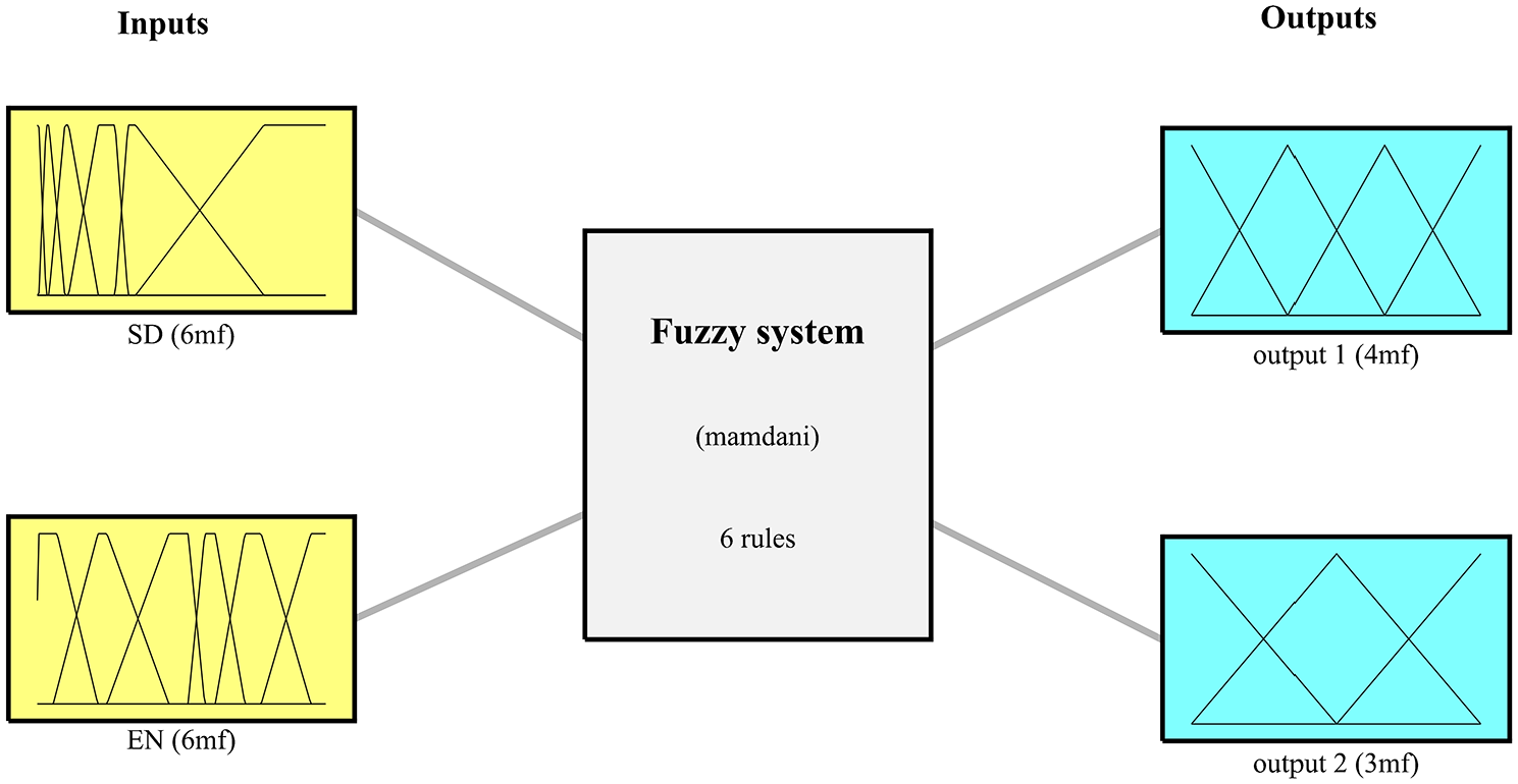
Fuzzy inference is composed of four essential parts: Fuzzification, rules, inference system and defuzzification, where the most used structure is Mamdani’s.⁴⁵ Figure 1 gives a short description about the main parts of the mamdani fuzzy system structure.

Figure 1.

Mamdani fuzzy process.

Fuzzification

In the fuzzification step, crisp values are converted to linguistic variables using the membership function that is used for input fuzzification in which the membership degree is between 0 and 1. A set of membership functions are given to the inputs fuzzification such as: trapezoidal, Gaussian, triangular, etc. where the choice of these functions depends on the problem solving strategy (reasoning). The trapezoidal and triangular membership functions are described by four boundary values and three values, respectively (Figure 2). Equations (8) and (9) define the membership’s degree of fuzzy sets between every boundary values.

trapezoidal = {\begin{matrix} 0 & if & x \leq a_{0} \\ \frac{x - a_{0}}{a_{1} - a_{0}} & if & a_{0} < x < a_{1} \\ 1 & if & a_{1} \leq x \leq a_{2} \\ \frac{a_{3} - x}{a_{3} - a_{2}} & if & a_{2} < x < a_{3} \\ 0 & if & x > a_{3} \end{matrix}

(8)

triangular = {\begin{matrix} 0 & if & x \leq a_{0} \\ \frac{x - a_{0}}{a_{1} - a_{0}} & if & a_{0} < x < a_{1} \\ 1 & if & x = a_{1} \\ \frac{a_{2} - x}{a_{2} - a_{1}} & if & a_{1} < x < a_{2} \\ 0 & if & x \geq a_{2} \end{matrix}

(9)

Figure 2.

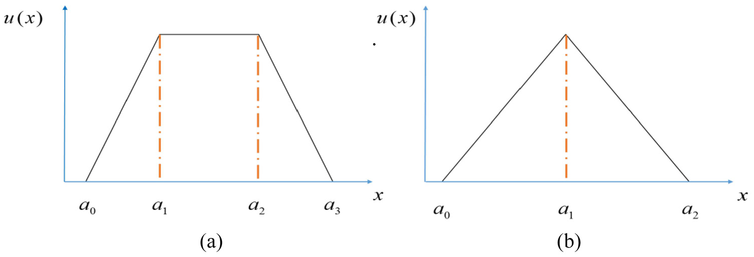
Trapezoidal (a) and triangular (b) membership functions.

Rules

Rules are the most important aspect of the classifier learning system, since they are based on each fuzzified membership input. These rules are defined using the IF-THEN expressions, for example if: x is A and y is B the output is C where x and y are the crisp inputs, A and B are the member inputs fuzzification and C is the member output fuzzification while the inference mechanism is used to process the sets of consequences to reach the output. Many operators exist, but the most preferred one is the min-max operator.

Defuzzification

In contrast to fuzzification, defuzzification converts the fuzzy output of the inference engine to a crisp value using membership functions similar to those used by fuzzifier. The center of gravity method is the most used technique for defuzzification as it averages the area of the resulting fuzzy sets using equation (10).

Z_{abssice} = \frac{\int f_{β} (z) . z dz}{\int f_{β} (z) dz}

(10)

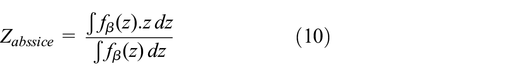
Figure 3 presents an example of defuzzification using the center of gravity procedure, where A₀, A₁, B₀ and B₁ are the fuzzy set memberships, Z₀ and Z₁ are the centers of gravity of the output memberships while y is the input value and z is the output value. Some algorithms used for defuzzification like the bisector of the surface, the mean of the maximum, the smallest of the maximum, the largest of the maximum are also presented in Figure 3.

Figure 3.

Example of FLS defuzzication method (center of gravity).

Experimental study

Test rig description

In order to confirm the efficiency of our proposed method using experimental vibration signals. Vibration data sets have been provided by the Case Western Reserve University Bearing Data Center.⁴⁶ Figure 4 presents the basic design of the used test bench, which is composed of a 2 horsepower (HP) Reliance electric motor that drives a shaft on which a torque sensor and an encoder are installed. The torque is applied to the shaft via a dynamometer and an electronic control system. For the tests, only the Drive end bearing (DE) is considered in our study and the ball bearing details are given in Table 1.

Figure 4.

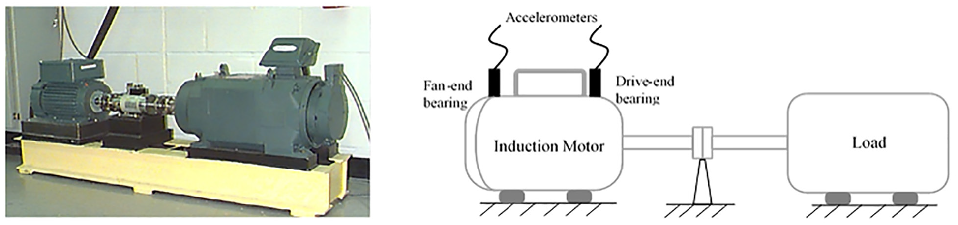
Experimental bearing test rig with a schematic illustration.

Table 1.

Bearing parameters.

Bearing type	Parameters
6205-2RSJEM SKF	Inside	0.9843
	Outside	2.0472
	Thickness	0.5906
	Ball	0.3126
	Pitch	1.537

Single point defects of 0.007 and 0.028 inches in the inner race (IR) and rolling element (B) and single point defects of 0.007 inches in the outer race (OR) were introduced separately into the test bearings by electro-discharge machining (EDM). Vibration data were recorded with a sampling frequency of 12 KHZ. Experimental signals have been collected for several work conditions under different loads and speeds (0 HP [1797 rpm], 1 HP [1772 rpm], 2 HP [1750 rpm], 3 HP [1723 rpm]) as shown in Table 2.

Table 2.

Works conditions.

Bearing state	Defect size(inches)	Speed(rpm)	Load(HP)
Healthy (H)	–	1797	0
		1772	1
		1750	2
		1723	3
Innerrace (IR)	0.007, 0.028	1797	0
		1772	1
		1750	2
		1723	3
Outerrace (OR)	0.007	1797	0
		1772	1
		1750	2
		1723	3
Rollingelement (B)	0.007, 0.028	1797	0
		1772	1
		1750	2
		1723	3

Experimental results and discussion

The data sets provided by Case Western Reserve University Bearing Data Center⁴⁶ will be used to evaluate the effectiveness and accuracy of our proposed approach for bearing diagnosis. Figure 5 displays the acceleration vibration signals recorded with healthy and three different OR, IR and B defects of 0.007 and 0.028 inches under 0 HP as load.

Figure 5.

Vibration signal of various bearing defects under 0 HP load and 1797 rpm speed.

Temporal analysis

When the rolling elements pass over the faulty areas, small impacts occur, producing mechanical shock waves in the time data. These small impacts excite the natural mechanical resonance frequencies in the motor. Whenever a defect affects other bearing parts, the same phenomena appear, and its repetition rate is equal to one of the characteristic defect frequencies (Tables 3 and 4). However, in Figure 5, we can clearly see that the three defects OR, IR and B with 0.007 and 0.028 inches do not have a significant impact on the vibration signal, since there is no significant increase in the time signal energy and no repetitive shock waves are observed at each revolution period. The measured signals can be very noisy, due to electrical and mechanical sources. This makes it even more difficult to detect incipient the defect. Therefore, it is practically impossible to detect the presence of faults by simply viewing the signals in time domain, since the fault impulses are masked by noise. Thus, a further analysis is required in this case since is difficult to identify the bearing defects from the time data.

Table 3.

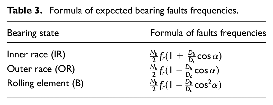
Formula of expected bearing faults frequencies.

Bearing state	Formula of faults frequencies
Inner race (IR)	$\frac{N_{b}}{2} f_{r} (1 + \frac{D_{b}}{D_{c}} \cos α)$
Outer race (OR)	$\frac{N_{b}}{2} f_{r} (1 - \frac{D_{b}}{D_{c}} \cos α)$
Rolling element (B)	$\frac{N_{b}}{2} f_{r} (1 - \frac{D_{b}}{D_{c}} \cos^{2} α)$

Table 4.

Theorical frequencies at load of 0 Hp and speed of 1797 rpm.

Bearing state	Fault frequency (Hz)
Healthy (H)	162.175
Inner race (IR)	107.37
Outer race (OR)	70.592
Rolling element (B)	11.929

Feature extraction based on TDFs and SVD

Our proposed method uses the TDFs-SVD combination to extract the defect feature in the feature extraction step while the FLS is used to automatically diagnose bearing failures. Experimental vibration signals with faultless and different bearing defects (OR, IR and B) under various loads as shown in the Table 2 are first divided into 270 groups of data sets using equation (11).

T_{sample} (s) = \frac{N_{t}}{N_{i}} • {f^{- 1}}_{sampling} = \frac{120000}{270} • 12 k^{- 1} = 0.03703

(11)

Where; N_t is the total signal length with 120,000 points, f_s is the sampling frequency and it is equal to 12KHZ while the initial matrix contains 270 N_i slices. The 270 slices are divided into 90 groups of three and each group of three is arranged in a row, so that in total we have a (90×3=270) matrix with every value in the matrix is in fact a signal slice (for instance x_1,1 is a signal slice). For six bearing states under various operating conditions, as shown in Table 2, we have in total 24 matrices of (90×3) presenting every case.

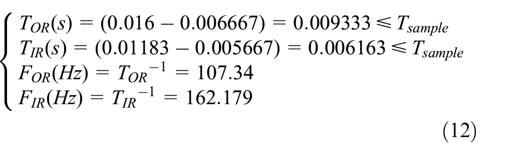
Figure 6 shows two time signal slices for OR (a) and IR (b) defects with 0.007 inches under no-load case with 1797 rpm. From Figure 6, the period of two successive maximum values is equal to the period obtained in equation (12). The obtained results match the theoretical frequencies in Table 4 avoiding by that any valuable information loss from the original signal.

{\begin{matrix} T_{OR} (s) = (0.016 - 0.006667) = 0.009333 \leq T_{sample} \\ T_{IR} (s) = (0.01183 - 0.005667) = 0.006163 \leq T_{sample} \\ F_{OR} (Hz) = {T_{OR}}^{- 1} = 107.34 \\ F_{IR} (Hz) = {T_{IR}}^{- 1} = 162.179 \end{matrix}

(12)

Figure 6.

Time vibration signal slices for OR (a) and IR (b) defects with 0.007 inches under 0 HP load and 1797 rpm speed.

Thereafter, entropy (EN) and standard deviation (SD) indicators are computed for each matrix obtained in the previous step in order to construct the feature matrix for each bearing state.

In order to avoid the dimensionality curse, SVD is then further used to reduce the dimensionality of the feature matrix and provide more stable vectors by extracting singular values for each bearing states under every working condition. The basis reason behind structuring the matrix in three columns is to limit the number of eigenvalues to three values. Finally, those three singular values will be selected to be used as inputs for the classifier system. Figures 7 and 8 give a better illustration about our proposed method.

Figure 7.

Flowchart of proposed method.

Figure 8.

Block diagram of proposed method.

Figures 9 and 10 show, respectively, the first, second and third singular values of the SD and EN feature matrices for the six different bearing states under variable speed and loads.

Figure 9.

Standard deviation features of the first, second and the third singular values.

Figure 10.

Entropy features of the first, second and the third singular values.

As shown in Figures 9 and 10, there is almost no overlapping between the six bearing states for all four speeds for the first singular values for both SD and EN. However, in the second and the third singular values almost all points overlap at every bearing states for the same speeds. From these figures, it appears that only the first singular values for both EN and SD are more stable and separable than the second and third singular values of the same indicators, which means that only the first singular values take ahead step in the feature classification, and it can be used to produce a new robust automatic classification method for bearing fault diagnosis.

In order to assess the impact of our proposed method before further investigation, a comparison is made between EN-SD and two of the most commonly used indicators; kurtosis (KU) and variance (VAR). Through the same feature extraction process, Figure 11 displays samples distribution using first singular value of EN-SD (a) and KU-VAR (b) are implemented in a two-dimensional representation. EN-SVD and SD-SVD features are plotted in Figure 11(a) respectively in the vertical and horizontal axes, while KU-SVD and VAR-SVD features are plotted in Figure 11(b).

Figure 11.

Distribution samples (EN-SD) (a) and (KU-VAR) (b) with first singular values.

As shown in Figure 11, KU-VAR sample distribution using the first singular value gives a mixed states sample (the healthy sample with a 0.007 inch ball defect) while the EN-SD gives more appreciable results without any confusion. Moreover, the defects separability is highly satisfactory which will facilitate the input fuzzification.

Figure 12 shows another comparison between EN-SD and KU-VAR, but this time, the second singular values are plotted. As shown in Figure 12 and as mentioned previously, a poor feature extraction results using the second singular values have been obtained, which explains the decision of using only the first singular values for further analysis, since they are more appropriate for bearing fault diagnosis.

Figure 12.

Distribution samples (EN-SD) (a) and (KU-VAR) (b) with second singular values.

State classification based on fuzzy logic system (FLS)

In this session, the fault feature vectors obtained by TDFs-SVD are used to identify and classify the bearing states by using the FLS. The proposed approach is tested under 24 different operating modes with 6 different bearing states (Table 2). Each vibration signal is divided into 270 data sets. The 270 slices are divided into 90 groups of three, and each group of three is arranged in a row, so that in total we have a (90×3=270) matrix. Thereafter, entropy and standard deviation indicators are applied for every matrix in order to obtain the feature matrix for each bearing state. Afterward, SVD is then further used to reduce the dimensionality of the feature matrix and to provide more stable vectors by extracting singular values for each bearing states under every working condition. Only the first singular values will be selected to be used as inputs for the classifier system. Finally, the FLS classifier provides an excellent tool for detecting, identifying and classifying different bearing states, even under different working conditions using well-defined memberships. The selected features of the first singular values of SD and EN are chosen as inputs of fuzzy classifier system as indicated in Figure 13.

Figure 13.

Fuzzification of inputs.

The inputs are fuzzified on the trapezoidal membership function by calculating the min-max feature inputs as indicated in Figure 14. The choice of the trapezoidal function returns to a certain interval between the min-max input boundaries. The fuzzification of the inputs and outputs are presented in Figures 15 and 16, respectively.

Figure 14.

Details of inputs-fuzzification.

Figure 15.

Memberships type of inputs-fuzzification.

Figure 16.

Memberships type of outputs-fuzzification.

Our classification system has two outputs as shown in Figure 16; the first is fuzzified for four memberships (H,IR,OR,B) to identify the fault type, while the second is fuzzified for three memberships, healthy, defects with sizes of 0.007 and 0.028 inches. The second output is used to show the bearing defect severity. The data sets are divided into training data (30 % of data sets) and test data (70 % of data sets) to test the effectiveness of the proposed approach. Table 5 provides detailed information on training and testing data numbers while Figure 17 summarizes the classification section.

Table 5.

Testing and training data.

Bearing defect type	Training datasize (30%)	Testing datasize (70%)
Healthy (H)	36	84
Inner race (IR7)	36	84
Outer race (OR7)	36	84
Rolling element (B7)	36	84
Inner Race (IR28)	36	84
Rolling element (B28)	36	84
Total	216	504

Figure 17.

Classification part.

The rules defined for our model are listed as follow:

If EN is H and SD is H then: Output 1 is H Output 2 is H.

If EN is IR7 and SD is IR7 then: Output 1 is 0.007 Output 2 is IR.

If EN is OR7 and SD is OR7 then: Output 1 is 0.007 Output 2 is OR.

If EN is B7 and SD is B7 then: Output 1 is 0.007 Output 2 is B.

If EN is IR28 and SD is IR28 then: Output 1 is 0.028 Output 2 is IR.

If EN is B28 and SD is B28 then: Output 1 is 0.028 Output 2 is B.

Figure 18 shows the surface view of the first (a) and second (b) output; where the inputs are structured in X and Y axes and the output is in Z axis. The axis boundaries are defined from the fuzzification part of the input–output boundaries (crisp values).

Figure 18.

Surface view of the first (a) and the second (b) output.

Figure 19 shows the first output which is fuzzified for four memberships (H,IR,OR,B) to identify the bearing fault type while Figure 20 shows the second output which is fuzzified for three memberships, healthy, defects with 0.007 and 0.028 inch sizes. Figures 19 and 20 clearly show that in a noisy environment and even under different working conditions, especially in the no load case, all samples are correctly classified and the actual outputs meet the target output classes. Experimental results highlight the efficiency and the accuracy of our proposed approach, which is based on TDFs, SVD and FLS. Our method offers a high classification rate, which implies a good decision for bearing fault diagnosis, even under varying working conditions with several speeds and loads.

Figure 19.

Tested samples of the first output.

Figure 20.

Tested samples of the second output.

Recently, ANN has been extensively used for feature classification for its efficiency and accuracy. However, the major problem with machine learning methods is the small size of the databases, which affects the neural network performance. On the other hand, fuzzy logic integrates the learning process by using human (expert) logic to solve non-complex data. A comparative study with one of the most used ANN tools, multi-layer perceptron (MLP) neural network, is made to confirm the advantage of our hybrid method. The same datasets which are divided into training data (30% of the datasets) and test data (70% of the datasets) are taken as input to the neural network.

Figures 21 and 22 show the performance of MLP network for the first and the second outputs, respectively.

Figure 21.

Performance evaluation of proposed MLP Network for the first output.

Figure 22.

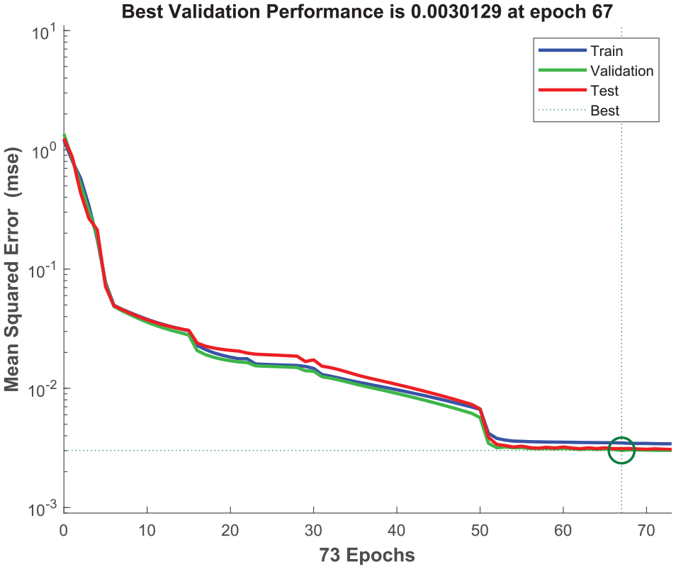
Performance evaluation of proposed MLP Network for the second output.

As shown in Figures 21 and 22, MLP offers a performance of 0.01638 Mean Squared Error (MSE) with 340 epochs for the first output and 0.0030129 MSE with 73 epochs for the second one. Clearly, FLS has an advantage over MLP in terms of classification accuracy (−1.5357e⁻⁴ for the first output and −2.7817e⁻⁴ for the second output). The obtained results illustrate the feasibility and efficiency of the proposed algorithm.

Conclusion

Bearing fault diagnosis using vibration analysis has been and remains widely used as a predictive maintenance strategy, since vibration signals carry a lot of valuable information that gives an insight about the health condition of an operating machine. However, vibration signals exhibit nonlinear and non-stationary behaviors buried in high background noise. This considerably increases the difficulty of defect detection, identification and classification using a conventional condition monitoring tool. Extracting bearing defect features require a robust automatic fault diagnosis technique for online inspection, a superb approach that could detect, identify and classify several bearing a defects especially under variable working condition with different speeds and loads. Therefore, a hybrid bearing fault diagnosis method has been developed in this paper to classify several bearing states from raw experimental vibration data. The proposed method combines between some TDFs tools and SVD for the feature extraction process and Fuzzy Logic System (FLS) for intelligent fault classification. Experimental results from the reference test bench provided by Case Wastern University (CWU) prove that our hybrid method is a reliable technique that shows great accuracy concerning the bearing failures classification even under different operating conditions.

Some future studies will be conducted to improve the field of bearing condition monitoring. For example, the proposed method has been studied for the case of different stable RPM therefore a natural extension of it will integrate an application to time-varying speed data.

Footnotes

Acknowledgements

The authors would like to thank the Solid Mechanics and Systems Laboratory (LMSS), University M’Hamed Bougara of Boumerdes, Faculty of Technology, Boumerdes, and the General Directorate for Scientific Research and Technological Development (DGRSDT), Algeria.

Handling Editor: James Baldwin

Declaration of conflicting interests

The author(s) declared no potential conflicts of interest with respect to the research, authorship, and/or publication of this article.

Funding

The author(s) received no financial support for the research, authorship, and/or publication of this article.

ORCID iDs

Fawzi Gougam

Chemseddine Rahmoune

References

Randall

. Vibration-based condition monitoring: industrial, aerospace and automotive applications. Chichester: John Wiley & Sons, 2011.

Ali

Fnaiech

Saidi

, et al. Application of empirical mode decomposition and artificial neural network for automatic bearing fault diagnosis based on vibration signals. Appl Acoust 2015; 89: 16–27.

Leite

GDNP

Araújo

Rosas

PAC

, et al. Entropy measures for early detection of bearing faults. Physica A 2019; 514: 458–472.

Lee

Ahn

. Mechanical vibration reduction control of two-mass permanent magnet synchronous motor using adaptive notch filter with fast Fourier transform analysis. IET Electric Power Appl 2012; 6: 455–461.

Tandon

Choudhury

. A review of vibration and acoustic measurement methods for the detection of defects in rolling element bearings. Tribol Int 1999; 32: 469–480.

Samuel

Pines

. A review of vibration-based techniques for helicopter transmission diagnostics. J Sound Vib 2005; 282: 475–508.

Terry

Lee

. What is the prognosis on your maintenance program. Eng Min J 1995; 196: 32.

Zhang

Zhi-Peng

. Application of iterative generalized short-time Fourier transform to fault diagnosis of planetary gearboxes. Chin J Eng 2017; 4: 16.

Wang

Zhao

, et al. Motor fault diagnosis based on short-time Fourier transform and convolutional neural network. Chin J Mech Eng 2017; 30: 1357–1368.

10.

Hartono

Halim

Wyn

. Gear fault diagnosis using an improved reassigned smoothed pseudo Wigner-Ville distribution. Cogent Eng 2018; 5: 1436928.

11.

Hartono

Dunant

Gethin

. Gear fault diagnosis using the general linear chirplet transform with vibration and acoustic measurements. J Low Freq Noise Vib Act Control 2019; 38: 36–52.

12.

Sharma

Avinash

Ram

. An empirical wavelet transform-based approach for cross-terms-free Wigner–Ville distribution. Signal Image Video Process 2020; 14: 249–256.

13.

Chen

Shen

Chen

, et al. Fault diagnosis method based on integration of RSSD and wavelet transform to rolling bearing. Measurement 2019; 131: 400–411.

14.

Malla

Rai

Kaul

, et al. Rolling element bearing fault detection based on the complex Morlet wavelet transform and performance evaluation using artificial neural network and support vector machine. Noise Vib Worldw 2019; 50: 313–327.

15.

Hoseinzadeh

Khadem

Sadooghi

. Modifying the Hilbert-Huang transform using the nonlinear entropy-based features for early fault detection of ball bearings. Appl Acoust 2019; 150: 313–324.

16.

Thakker

Dave

Vakharia

, et al. Fault diagnosis of ball bearing using Hilbert Huang transform and LASSO feature ranking technique. IOP Conf Ser Mater Sci Eng 2020; 841: 012006.

17.

Tian

Zhang

, et al. Application of an enhanced fast kurtogram based on empirical wavelet transform for bearing fault diagnosis. Meas Sci Technol 2019; 30: 035001.

18.

Liang

Zhao

Lin

, et al. A novel indicator to improve fast kurtogram for the health monitoring of rolling bearing. IEEE Sens J 2020; 20: 12252–12261.

19.

Die

Kang

Chi

. Rolling bearing fault feature extraction method based on VMD and fast-kurtogram. In: 2019 IEEE 3rd information technology, networking, electronic and automation control conference (ITNEC), Chengdu, China, 15–17 March 2019, pp.2088–2092. New York: IEEE.

20.

Moshrefzadeh

Fasana

. The Autogram: an effective approach for selecting the optimal demodulation band in rolling element bearings diagnosis. Mech Syst Signal Process 2018; 105: 294–318.

21.

Afia

Rahmoune

Benazzouz

. Gear fault diagnosis using Autogram analysis. Adv Mech Eng 2018; 10: 1687814018812534.

22.

Gougam

Rahmoune

Benazzouz

, et al. Health monitoring approach of bearing: application of adaptive neuro fuzzy inference system (ANFIS) for RUL-estimation and Autogram analysis for fault-localization. In: 2020 prognostics and health management conference (PHM-Besançon), Besancon, 4–7 May 2020, pp.200–206. New York: IEEE.

23.

Afia

Rahmoune

Benazzouz

, et al. New intelligent gear fault diagnosis method based on Autogram and radial basis function neural network. Adv Mech Eng 2020; 12: 1–14.

24.

Zair

Rahmoune

Benazzouz

. Multi-fault diagnosis of rolling bearing using fuzzy entropy of empirical mode decomposition, principal component analysis, and SOM neural network. Proc IMechE, Part C: J Mech Eng Sci 2019; 233: 3317–3328.

25.

Zair

Rahmoune

Benazzouz

, et al. Automatic condition monitoring of electromechanical system based on MCSA, spectral kurtosis and SOM neural network. J Vibro Eng 2019; 21: 2082–2095.

26.

Afia

Rahmoune

Benazzouz

, et al. New gear fault diagnosis method based on MODWPT and neural network for feature extraction and classification. J Test Eval. Epub ahead of print 14 June 2019. DOI: 10.1520/JTE20190107.

27.

Huang

. Ensemble empirical mode decomposition: a noise-assisted data analysis method. Adv Adapt Data Anal 2009; 1: 1–41.

28.

Mahgoun

Bekka

Felkaoui

. Gearbox fault diagnosis using ensemble empirical mode decomposition (EEMD) and residual signal. Mech Ind 2012; 13: 33–44.

29.

Zhao

Sun

Deng

, et al. A new feature extraction method based on EEMD and multi-scale fuzzy entropy for motor bearing. Entropy 2017; 19: 14.

30.

Afia

Rahmoune

Benazzouz

. An early gear fault diagnosis method based on RLMD, Hilbert transform and cepstrum analysis. Mech Syst Control 2020.

31.

Liu

, et al. Crack fault detection for a gearbox using discrete wavelet transform and an adaptive resonance theory neural network. J Mech Eng 2015; 61: 63–73.

32.

Heydarzadeh

Kia

Nourani

, et al. Gear fault diagnosis using discrete wavelet transform and deep neural networks. In: IECON 2016-42nd annual conference of the IEEE industrial electronics society, Florence, 23–26 October 2016, pp.1494–1500. New York: IEEE.

33.

Er-raoudi

Diany

Aissaoui

, et al. Gear fault detection using artificial neural networks with discrete wavelet transform and principal component analysis. J Mech Eng Sci 2016; 10: 2016–2029.

34.

Bajric

Zuber

Skrimpas

, et al. Feature extraction using discrete wavelet transform for gear fault diagnosis of wind turbine gearbox. Shock Vib 2016; 2016: 6748469.

35.

Bellman

. Adaptive control processes: a guided tour, vol. 2045. Princeton, NJ: Princeton University Press, 2015.

36.

, et al. Design a degradation condition monitoring system scheme for rolling bearing using EMD and PCA. Ind Manag Data Syst 2017; 117: 713–728.

37.

Patel

Agrawal

Giri

. Induction motor bearing fault classification using PCA and ANN. In: Giri

Verma

Patel

, et al. (eds) Computing algorithms with applications in engineering. Singapore: Springer, 2020, pp.269–284.

38.

Merainani

Rahmoune

Benazzouz

, et al. A novel gearbox fault feature extraction and classification using Hilbert empirical wavelet transform, singular value decomposition, and SOM neural network. J Vib Control 2018; 24: 2512–2531.

39.

Chemseddine

Boualem

Djamel

, et al. Gear fault feature extraction and classification of singular value decomposition based on Hilbert empirical wavelet transform. J Vibro Eng 2018; 20: 1603–1618.

40.

Gougam

Rahmoune

Benazzouz

, et al. Bearing fault diagnosis based on feature extraction of empirical wavelet transform (EWT) and fuzzy logic system (FLS) under variable operating conditions. J Vibro Eng 2019; 21: 1636–1650.

41.

Krishnakumari

Elayaperumal

Saravanan

, et al. Fault diagnostics of spur gear using decision tree and fuzzy classifier. Int J Adv Manuf Technol 2017; 89: 3487–3494.

42.

Sharma

Parey

. A review of gear fault diagnosis using various condition indicators. Procedia Eng 2016; 144: 253–263.

43.

Hemba

Islam

. Fuzzy logic: a review. Int J Comput Sci Eng 2017; 5: 61–63.

44.

Kasbe

Pippal

. Dengue fever: state-of-the-art symptoms and diagnosis. Int J Comput Sci Eng 2016; 4: 26–30.

45.

Dadios

(ed). Fuzzy logic controls, concepts, theories and applications. BoD-Books on Demand, 2012, pp.325–350.

46.

Loparo

. Case western reserve university bearing data center. Bearings Vibration Data Sets, Case Western Reserve University, 2012, pp.22–28. http://csegroups.case.edu/bearingdatacenter/home

Bearing faults classification under various operation modes using time domain features,singular value decomposition,and fuzzy logic system

Abstract

Keywords

Introduction

Mathematical background

Feature extraction based on temporal analysis

Singular value decomposition

Fuzzy logic system

Fuzzification

Rules

Defuzzification

Experimental study

Test rig description

Experimental results and discussion

Temporal analysis

Feature extraction based on TDFs and SVD

State classification based on fuzzy logic system (FLS)

Conclusion

Footnotes

Acknowledgements

Declaration of conflicting interests

Funding

ORCID iDs

References