A hybrid time-frequency information-based method for bearing fault diagnosis

Abstract

Rolling bearing vibration signals are inherently non-stationary and exhibit complementary fault-related characteristics across time and frequency domains. Effectively modeling such heterogeneous information remains a key challenge for robust fault diagnosis under complex operating conditions. To address this issue, this study proposes a hybrid fault diagnosis framework based on parallel dual-channel feature extraction and Transformer-based early fusion. In the proposed architecture, raw vibration signals are simultaneously processed by a time-domain branch and a frequency-domain branch, enabling the preservation of domain-specific characteristics without sequential information loss. By performing feature fusion at an early stage, the Transformer encoder is able to capture global dependencies and cross-domain interactions through self-attention, thereby enhancing discriminative capability and robustness in noisy environments. Experimental results on the Case Western Reserve University (CWRU) dataset demonstrate that the proposed method achieves a classification accuracy of 99.99%. Furthermore, cross-dataset validation on the XJTU-SY bearing dataset, together with noise robustness and ablation studies, confirms the effectiveness, generalization ability, and structural rationality of the proposed parallel time–frequency fusion strategy. These findings indicate that the proposed framework provides a reliable and practical solution for rolling bearing fault diagnosis in real-world industrial scenarios.

Introduction

Rolling bearings are fundamental support components in rotating machinery, and their operational condition critically affects system performance, reliability, and safety. ¹ Owing to long-term exposure to high loads, strong vibrations, and harsh operating environments, bearing faults may gradually evolve and, if not detected in time, can lead to unexpected downtime, economic losses, and even catastrophic failures. ² Predictive Maintenance (PdM) aims to mitigate these risks by enabling early fault detection and condition-aware maintenance through real-time monitoring and data-driven analysis. ³ Consequently, achieving accurate and robust bearing fault diagnosis has become a central research topic in both academia and industry. ⁴

Existing bearing health monitoring methods can be broadly categorized into physical model-based and data-driven approaches. ⁵ Physical model-based methods rely on mechanical principles and degradation mechanisms to establish diagnostic or prognostic models. For example, Chen et al. ⁶ proposed a sequential model for gas turbine performance evaluation, while Zhang et al. ⁷ developed a reliability model for solid-lubricated bearings using Copula-based dependency modeling. Kumar et al. ⁸ introduced an entropy-based state-space model for degradation monitoring and remaining useful life (RUL) estimation, and Yu et al. ⁹ improved fatigue life prediction by compensating material sensitivity in the Smith–Watson–Topper (SWT) model. Cui et al. ¹⁰ further proposed a switching unscented Kalman filter for bearing condition assessment and RUL prediction. Although these approaches can achieve high accuracy under well-defined assumptions, they typically require extensive domain knowledge and exhibit limited adaptability to complex operating conditions and diverse fault modes. ¹¹

To overcome these limitations, data-driven methods—particularly deep learning-based techniques—have gained increasing attention. ¹² By directly learning discriminative features from high-dimensional sensor data, deep learning models avoid explicit physical modeling and demonstrate strong representation capability. Recent studies include Visual Transformer models enhanced by meta-learning, ¹³ GAN-based frameworks for data augmentation, ¹⁴ multiscale CNN architectures leveraging time–frequency features, ¹⁵ CNN–LSTM hybrids for sequential modeling, ¹⁶ STFT-based image representations combined with CNNs, ¹⁷ and probabilistic Transformer frameworks for uncertainty-aware diagnosis. ¹⁸ In addition, recent complexity-based methods have also been advanced for bearing diagnosis, such as multivariate Rating Entropy and multivariate variable-step multiscale EDELZC-based Lempel–Ziv complexity, which enhance robustness by modeling multi-channel dependencies and multi-scale nonlinear dynamics.^19,20

Despite their promising performance, existing deep learning approaches still face significant challenges when applied to real-world bearing fault diagnosis. On one hand, time-domain models are effective at capturing transient impulses and local temporal patterns but are highly sensitive to noise and operating condition variations. On the other hand, frequency-domain approaches emphasize fault characteristic frequencies and spectral structures, yet may suffer from information loss under strong noise or nonstationary conditions. Critically, many existing methods rely on sequential transformations (e.g. generating spectrograms as input), where one domain is fundamentally constrained by the pre-processing artifacts of the other. Such architectural dependency inevitably introduces representation bias and may lead to the loss of weak, domain-specific fault signatures under low signal-to-noise ratio (SNR) conditions.

Recent experimental evidence further reveals that the degradation mechanisms of time-domain and frequency-domain features under noise are inherently different. When exposed to increasing noise intensity, models relying solely on time-domain or frequency-domain features exhibit substantial performance degradation, whereas architectures that preserve and integrate complementary information from both domains demonstrate superior robustness. These observations indicate that effective bearing fault diagnosis, particularly under noisy and complex environments, requires a representation learning strategy capable of simultaneously capturing transient temporal signatures and stable spectral characteristics.

Motivated by this insight, this study proposes a hybrid fault diagnosis framework based on parallel time–frequency dual-domain feature extraction and Transformer-based fusion. Instead of sequentially transforming and fusing features, the proposed method processes raw vibration signals through two parallel channels: a time-domain channel that extracts localized temporal features directly from raw signals, and a frequency-domain channel that learns discriminative spectral representations from STFT-based time–frequency maps. A Transformer encoder is then employed to model global dependencies and cross-domain interactions between the extracted features, enabling comprehensive fault representation under varying noise levels and operating conditions.

The main contributions of this work are summarized as follows:

• (1) Parallel dual-domain feature extraction mechanism: A time–frequency parallel architecture is designed to preserve the pristine domain-specific fault characteristics and avoid information loss associated with single-domain or sequential fusion strategies.

• (2) Transformer-based cross-domain fusion: A Transformer encoder is introduced to capture global dependencies and interactions between time-domain and frequency-domain features, enhancing robustness and discriminability under noisy conditions.

• (3) Comprehensive experimental validation: Extensive experiments on the CWRU and XJTU-SY bearing datasets, including noise robustness analysis and ablation studies, demonstrate that the proposed framework achieves superior diagnostic accuracy and stability compared to single-domain and partially fused models.

The remainder of this paper is organized as follows. Section “Background” introduces the theoretical background and overall framework of the proposed method. Section “Experiments” presents experimental evaluations and performance analysis. Section “Conclusion” concludes the paper and discusses future research directions.

Background

The non-stationary and complex frequency characteristics of rolling bearing vibration signals make time-frequency analysis methods particularly well-suited for fault detection. The STFT preserves both temporal and key spectral information, effectively revealing the correspondence between characteristic fault frequencies and specific bearing defects. This facilitates more accurate identification and assessment of fault conditions. Within the proposed framework, CNN are utilized to extract localized features from the STFT spectrogram, while Transformers are employed to capture long-range dependencies and complex patterns. This complementary integration of spatial and temporal features significantly enhances diagnostic accuracy.

STFT

The STFT is a method used to analyze the time-frequency characteristics of non-stationary signals by segmenting the signal and applying the Fourier Transform to each segment. The fundamental process involves multiplying the original signal s(t) by a window function $w(t-\tau )$ , which is t shifted along the time axis to extract local segments of the signal. Each windowed segment is then transformed using the Fourier Transform, producing a time-frequency representation. The formal definition of the STFT is given by:

$$T(\tau ,\xi )={\int }_{-\infty }^{+\infty }s(t)w^{*}(t-\tau )e^{-j2\pi \xi t}\mathrm{dt}$$

(1)

where s(t) is the original signal, $w(t-\tau )$ is the window function centered at time τ and $w^{*}(·)$ is its complex conjugate, ξ is the frequency variable; and $T(\tau ,\xi )$ is the complex amplitude of the signal at time τ and frequency ξ.

CNN

Convolutional Neural Networks (CNNs) are a class of deep learning models widely used in computer vision tasks such as image classification, object detection, and semantic segmentation. ²¹ They achieve efficient feature extraction and pattern recognition by mimicking the hierarchical processing characteristics of the biological visual cortex. ²² As a type of feed-forward neural network, a CNN extracts features from input data through a sequence of convolutional, activation, pooling, and fully connected layers. The overall structure of a CNN is illustrated in Figure 1.

Figure 1.

CNN structure.

The convolutional layer is the core component of CNN, where the convolution operation serves as the primary mechanism for local feature extraction. Depending on the dimensionality of the input data, CNNs can be implemented in either one-dimensional or two-dimensional forms to accommodate different types of signals or images.

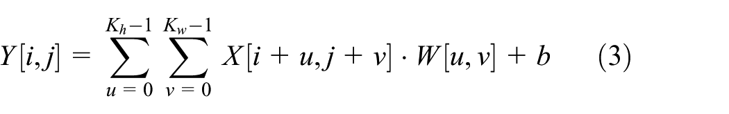
For one-dimensional input signals, such as time-series vibration waveforms, a one dimension CNN applies a learnable filter $w\in {\mathbb{R}}^K$ along the temporal axis, where K denotes the kernel size. Given an input sequence $x\in {\mathbb{R}}^N$ , the output $y[i]$ at temporal position i is computed as:

$$y[i]=\sum _{j=0}^{K-1}x[i+j]·w[j]+b$$

(2)

where $x[i+j]$ is the input signal at position $i+j$ , $w[j]$ represents the j-th weight of the kernel, and b is a scalar bias term. This operation enables end-to-end feature extraction directly in the time domain, effectively capturing local temporal characteristics such as transients and periodic harmonics.

In contrast, for two-dimensional inputs, such as spectrograms generated by STFT, a 2D CNN applies a two-dimensional filter $W\in {\mathbb{R}}^{K_h\times K_w}$ across the spatial dimensions of the input. Given an input map $X\in {\mathbb{R}}^{H\times W}$ , where H and W denote the height and width respectively, the convolution output $Y[i,j]$ at spatial position (i, j) is defined as:

$$Y[i,j]=\sum _{u=0}^{K_h-1}\sum _{v=0}^{K_w-1}X[i+u,j+v]·W[u,v]+b$$

(3)

where $X[i+u,j+v]$ represents the input value at position $(i+u,j+v)$ , $W[u,v]$ is the filter weight at index (u, v), and b is the scalar bias term. The 2D convolution facilitates learning of localized frequency–time dependencies, making it particularly effective in processing image-like data or time–frequency representations such as spectrograms.

Both one-dimensional (1D) and two-dimensional (2D) CNN architectures leverage the principles of weight sharing and hierarchical feature learning. These characteristics not only reduce the number of trainable parameters but also enhance the model’s generalization capability across varying input distributions by progressively capturing higher-level abstractions through successive layers.

Following each convolutional operation, a nonlinear activation function is applied to enable the network to learn complex, non-linear relationships. One of the most commonly used activation functions is the Rectified Linear Unit (ReLU), defined as:

$$f(x)=max(0,x)$$

(4)

where, x represents the outputs from the convolutional layer. Activation functions enable the network to learn complex, non-linear relationships within the data.

Pooling layers, often succeeding convolutional layers, serve to reduce the spatial dimensions of feature maps and enhance model robustness. For an input feature map F, the max pooling operation over a region ${\mathcal{R}}_{\mathrm{ij}}$ can be formulated as:

$$P_{\mathrm{ij}}=\underset{(r,c)\in {\mathcal{R}}_{\mathrm{ij}}}{max}{F}_{(r,c)}$$

(5)

where P _ij is the value of the pooled feature map at position $(i,j)$ , and ${\mathcal{R}}_{\mathrm{ij}}$ is the pooling region in the input feature map corresponding to the output position $(i,j)$ . Max pooling selects the maximum value within each region, effectively reducing feature map size and improving translation invariance.

After multiple convolutional and pooling layers, the feature maps are flattened and fed into fully connected layers. These layers perform linear transformations and non-linear activations to map the extracted features to the output space. The output z of a fully connected layer can be represented as:

$$z=\phi (\mathrm{Ua}+c)$$

(6)

where a is the input vector, U is the weight matrix, c is the bias vector, and φ is the activation function. In classification tasks, the final fully connected layer typically employs a Softmax function to convert outputs into probability distributions.

By stacking convolutional layers, activation functions, pooling layers, and fully connected layers, CNNs are able to construct deep network architectures capable of automatically learning hierarchical feature representations directly from raw input data.

Transformer model

Transformer models have fundamentally reshaped the processing of sequential data by introducing self-attention mechanisms, which enable efficient and accurate modeling of long-range dependencies. ²³ The Transformer architecture consists of an encoder and a decoder, each comprising multiple stacked layers without parameter sharing. Through the integration of multi-head self-attention mechanisms and position-wise feedforward networks—along with residual connections and layer normalization—the Transformer is capable of capturing complex, long-range contextual relationships within sequences. The overall architecture of the Transformer is illustrated in Figure 2.

Figure 2.

Transformer structure.

At the input stage, the Transformer model employs an embedding layer to map discrete tokens into continuous vector representations suitable for downstream processing. To preserve the sequential nature of the input—since the model lacks inherent convolution—positional encodings are added to the embeddings. These encodings inject information about the position of each token in the sequence. A common approach is to use sinusoidal functions to generate fixed positional encodings, defined as follows:

$${\mathrm{PE}}_{(\mathrm{pos},2i)}=\sin \left(\frac{\mathrm{pos}}{{\alpha }^{2i/d_{mod\mathrm{el}}}}\right)$$

(7)

$${\mathrm{PE}}_{(\mathrm{pos},2i+1)}=\cos \left(\frac{\mathrm{pos}}{{\alpha }^{2i/d_{mod\mathrm{el}}}}\right)$$

(8)

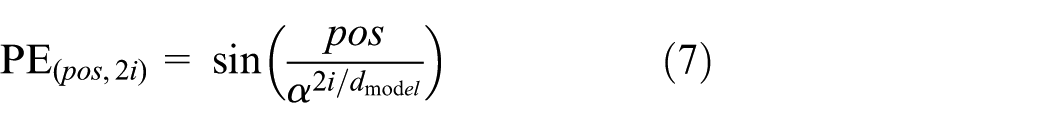
where pos denotes the position index, i is the dimensional index, $d_{mod\mathrm{el}}$ the dimension of the embeddings. These functions ensure each position has a unique encoding and that the relative distances between positions are preserved across the sequence.

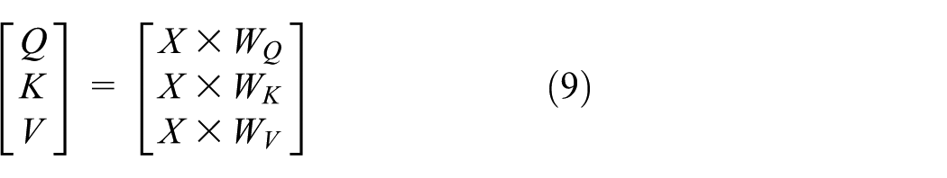
In the encoder, each layer first applies a multi-head self-attention mechanism to learn the inter-dependencies among different positions of the input sequence. Concretely, given an input matrix X, it produces query Q, key K, and value V vectors via trainable weight matrices:

$$\left[\begin{array}{c}Q\hfill \\ \multicolumn{1}{c}{K}\\ \multicolumn{1}{c}{V}\end{array}\right]=\left[\begin{array}{c}X\times W_Q\hfill \\ \multicolumn{1}{c}{X\times W_K}\\ \multicolumn{1}{c}{X\times W_V}\end{array}\right]$$

(9)

Next, the dot-product attention scores are computed, scaled, and normalized, serving as the foundation for the subsequent attention mechanism. The matrix of outputs as:

$$\mathrm{Attention}(Q,K,V)=\mathrm{Softmax}\left(\frac{Q{K}^T}{\sqrt{d_k}}\right)V$$

(10)

where d _k is the dimensionality of the key vectors. Multi-head attention executes this process in parallel across multiple subspaces, thereby enabling the modeling of diverse semantic relationships The output of the attention layer is added back to the original input through a residual connection, followed by layer normalization.

$$\begin{array}{c}\mathrm{MultiHead}(Q,K,V)=\mathrm{Concat}({\mathrm{head}}_1,\dots ,{\mathrm{head}}_{\mathrm{h}})W^O\hfill \\ \mathrm{where}{\mathrm{head}}_{\mathrm{i}}=\mathrm{Attention}({\mathrm{QW}}_i^Q,{\mathrm{KW}}_i^K,{\mathrm{VW}}_i^V)\hfill \end{array}$$

(11)

where $W_i^Q\in {\mathbb{R}}^{d_{\mathrm{model}}\times d_k}$ , $W_i^K\in {\mathbb{R}}^{d_{\mathrm{model}}\times d_k}$ , $W_i^V\in {\mathbb{R}}^{d_{\mathrm{model}}\times d_v}$ , and $W_i^V\in {\mathbb{R}}^{d_{\mathrm{model}}\times d_v}$ $W^O\in {\mathbb{R}}^{d_{\mathrm{model}}\times h{d}_v}$ .

A two-layer feedforward network further transforms the resulting features, often expressed as:

$$\mathrm{FFN}(z)=max\left(\begin{array}{cc}0,\hfill & z{W}_1+b_1\hfill \end{array}\right)W_2+b_2.$$

(12)

In the decoder, the structure mirrors that of the encoder, but the self-attention layer is masked to avoid accessing future positions, and an additional cross-attention layer leverages encoder outputs as keys and values. A linear–softmax layer maps the final decoder output onto the vocabulary space to generate a distribution over the target sequence.

Proposed model

This section presents a novel CNN–Transformer-based fault diagnosis framework designed to capture both local and long-range dependencies in rolling bearing vibration signals. As shown in Figure 3, the model comprises three key components: (1) a time-domain CNN channel that extracts local temporal features directly from raw signals to preserve the precise arrival times of transient impulsive shocks caused by localized defects; (2) a SpectralCNN module, where the STFT converts the raw signal into spectrograms, from which frequency-domain CNNs extract stabilized spectral signatures and cyclostationary energy distributions; and (3) a Transformer encoder that fuses these extracted features. By maintaining parallel dual-channels rather than a single sequential transformation, the framework avoids the “temporal smearing” effect inherent in fixed-window spectral analysis, ensuring that the Transformer can model cross-modal interactions between high-resolution transients and frequency-domain harmonics. Finally, a fully connected layer generates the classification output. Finally, a fully connected layer generates the classification output.

Figure 3.

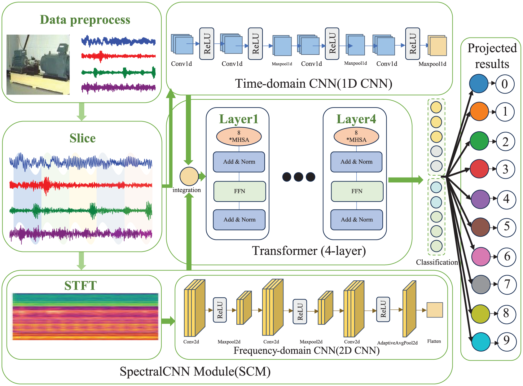
CNN-transformer structure.

This dual-channel architecture, augmented by the self-attention mechanism of the Transformer, effectively integrates both local and global fault-related information. Compared to conventional single-channel CNN or Transformer-only approaches, the proposed framework offers enhanced diagnostic accuracy.

The first channel focuses on processing raw vibration signals in the time domain. Given an input signal of length L, the data is passed through a series of one-dimensional (1D) convolutional and pooling layers to extract localized temporal features. Each convolutional layer employs carefully selected kernel sizes and strides, determined based on the sampling frequency and the dominant fault-related frequency bands. As the network depth increases, the number of feature channels is progressively expanded, enabling the extraction of increasingly abstract representations associated with different fault types. Finally, a global pooling layer aggregates the learned features into a compact vector representation, denote as $v_{\mathrm{temporal}}\in {\mathbb{R}}^{D_1}$ .

The same vibration signal is transformed into a frequency representation via the STFT. The output is a 2D image of dimension F×T, where F and T represent the frequency and temporal axes, respectively. This image is processed by a 2D CNN module comprising multiple convolutional layers with nonlinear activations. Similar to the time-domain channel, global average pooling (or adaptive average pooling) is applied to yield a frequency-domain feature vector $v_{\mathrm{freq}}\in {\mathbb{R}}^{D_2}$ .

After extracting the temporal- and frequency-domain features, these features are concatenated along the feature dimension:

$$v_{\mathrm{concat}}=[v_{\mathrm{temporal}}\parallel v_{\mathrm{freq}}]$$

(13)

leading to a unified embedding of dimension $D=D_1+D_2$ . The concatenated feature vector is subsequently reformatted as a sequence input—or retained as a single token, depending on the design—for processing by the Transformer encoder. The encoder consists of multiple identical layers, each comprising a multi-head self-attention (MHSA) mechanism followed by a position-wise feed-forward network (FFN). To stabilize training and facilitate efficient gradient propagation, residual connections and layer normalization are applied after each sub-layer.

The output of the Transformer encoder is then aggregated: if the encoder produces a sequence of tokens, global average pooling is applied; if a single token representation is used, the output is taken directly. The resulting fixed-size feature vector z is then passed through a fully connected layer:

$$\hat{y}=\mathrm{Softmax}(W·z+b)$$

(14)

where W and b are learnable parameters. $\hat{y}$ denotes the predicted probability distribution over the fault categories. During the training phase, a cross-entropy loss function is minimized to enhance classification accuracy.

Experiments

Data description

To evaluate the performance of the proposed fault diagnosis method, this study utilizes the publicly available bearing dataset from Case Western Reserve University (CWRU). ²⁴ The data acquisition setup is illustrated in Figure 4. Single-point faults were artificially induced in SKF 6205-2RS JEM deep-groove ball bearings using electro-discharge machining (EDM), generating defects on the inner race (IR), outer race (OR), and rolling elements (Ball) with three damage sizes: 0.1778, 0.3556, and 0.5334 mm. The test rig operated at a motor speed of approximately 1772 rpm, and vibration signals were captured by an accelerometer mounted on the fan end (FE) at a sampling rate of 12 kHz.

Figure 4.

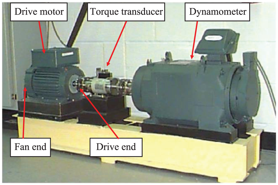
The test stand of CWRU.

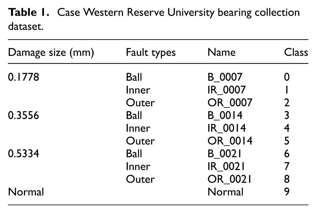
In this study, three fault types—inner race (IR), outer race (OR), and ball fault (BF)—along with a normal condition are considered, resulting in a total of 10 distinct health states. Detailed information on these states is provided in Table 1. Based on the available data volume and quality, each fault category is assigned 500 samples, with 400 used for training and 100 for testing, following a 4:1 split. This yields a total of 5000 samples. Each sample comprises 1024 data points to capture sufficient fault-related features. All experiments are conducted using the PyTorch deep learning framework on a workstation equipped with an AMD Ryzen 7 5800H CPU (8 cores, 3.20 GHz), an NVIDIA GeForce RTX 3060 Laptop GPU (6 GB VRAM), and 16 GB of DDR4 RAM. To ensure robustness and eliminate randomness, each experiment is repeated multiple times, and the average performance is reported as the final result.

Table 1.

Case Western Reserve University bearing collection dataset.

Damage size (mm)	Fault types	Name	Class
0.1778	Ball	B_0007	0
	Inner	IR_0007	1
	Outer	OR_0007	2
0.3556	Ball	B_0014	3
	Inner	IR_0014	4
	Outer	OR_0014	5
0.5334	Ball	B_0021	6
	Inner	IR_0021	7
	Outer	OR_0021	8
Normal		Normal	9

The XJTU-SY rolling bearing dataset was provided by the Institute of Design Science and Basic Component Research, Xi’an Jiaotong University. The bearing test rig used to construct the dataset is shown in Figure 5. Three operating conditions with different rotational speeds and radial loads were considered in the experiments, namely 2100 rpm (35 Hz) with 12 kN load, 2250 rpm (37.5 Hz) with 11 kN load, and 2400 rpm (40 Hz) with 10 kN load. For each operating condition, five different fault types were introduced, resulting in a total of 15 complete bearing fault scenarios. All vibration signals were obtained through multiple accelerated degradation experiments, which record the full degradation process of rolling bearings from healthy state to failure. In this study, only the five fault types under the operating condition of 35 Hz were selected for analysis. The XJTU-SY dataset provides two vibration channels, including vertical and horizontal vibration signals.

Figure 5.

The test stand of XJTU-SY.

Evaluation indicators

To assess the performance of the proposed fault diagnosis model, five evaluation metrics are employed: Accuracy (ACC), Precision (PRE), Recall (REC), F1 Score, and Area Under the Curve (AUC). In comparing the model’s predictions with the ground truth, four possible outcomes are considered: True Positive (TP), False Positive (FP), False Negative (FN), and True Negative (TN). Based on these outcomes, the evaluation metrics are defined as follows.

ACC measures the overall correctness of the model’s predictions. It is given by

$$\mathrm{ACC}=\frac{\mathrm{TP}+\mathrm{TN}}{\mathrm{TP}+\mathrm{TN}+\mathrm{FP}+\mathrm{FN}}$$

(15)

PRE focuses on the proportion of true positives among the predicted positives:

$$\mathrm{PRE}=\frac{\mathrm{TP}}{\mathrm{TP}+\mathrm{FP}}$$

(16)

REC, also known as sensitivity, gauges the proportion of actual positive instances correctly identified:

$$\mathrm{REC}=\frac{\mathrm{TP}}{\mathrm{TP}+\mathrm{FN}}$$

(17)

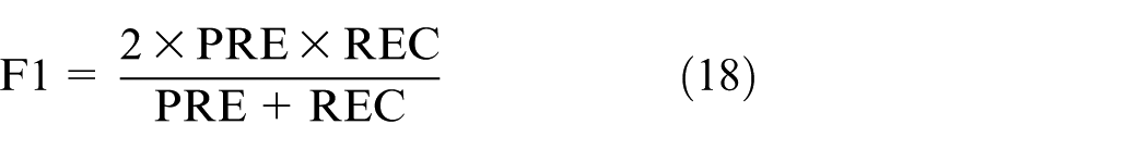
The F1 Score is the harmonic mean of Precision and Recall, balancing both metrics:

$$\mathrm{F}1=\frac{2\times \mathrm{PRE}\times \mathrm{REC}}{\mathrm{PRE}+\mathrm{REC}}$$

(18)

The AUC typically refers to the area under the Receiver Operating Characteristic (ROC) curve, which reflects the model’s overall discriminative capability across various threshold settings. A value closer to 1 indicates superior classification performance.

In summary, Accuracy measures the model’s overall correctness; Precision and Recall emphasize the correctness of positive predictions and the completeness of detecting actual positives, respectively; the F1 Score provides a harmonic balance between Precision and Recall; and AUC evaluates performance across multiple decision thresholds. By jointly considering these metrics, a more comprehensive and reliable assessment of the fault diagnosis model’s performance can be achieved.

Data process

The classification of bearing conditions is based on the fault location and the corresponding fault diameter. Ten distinct health states are defined accordingly. The following figures present the time-domain and frequency-domain waveforms corresponding to each of these state categories.

As shown in Figure 6, the time-domain and frequency-domain vibration signals of the bearing under normal operating conditions exhibit stable characteristics. The time-domain waveform shows moderate amplitude oscillations around a constant baseline. In the corresponding frequency spectrum, a dominant peak appears near 1000 Hz with an amplitude of approximately 0.02, and no additional significant peaks are observed, indicating the absence of defect-induced resonances.

Figure 6.

Fan-end bearing under healthy condition.

As shown in Figure 7, the data include nine sets of time–frequency plots corresponding to bearings with various localized defects and severities. Compared to the normal bearing, most faulty conditions exhibit increased time-domain amplitude, indicating more intense mechanical impacts. In the frequency domain, the dominant component near 1000 Hz typically remains, while additional peaks and sidebands frequently emerge in the 1500–2000 Hz range and occasionally beyond 3000 Hz. The elevated magnitudes of these components (often exceeding 0.03) reflect the increased energy associated with spalling, cracking, or other fault mechanisms within the bearing elements.

Figure 7.

Fan-end bearing under fault condition.

The vibration signals in the dataset are transformed into two-dimensional time–frequency image samples using the STFT. These images are subsequently used as input for the transformer network. As illustrated in Figure 7, the dataset encompasses image representations of rolling bearings in 10 distinct operational states.

As shown in Figure 8, the images extracted from vibration signals under different operating conditions exhibit increasingly pronounced banded structures. Specifically, as the fault severity increases, brighter horizontal or vertical stripes appear more prominently in the mid- to high-frequency regions, indicating localized energy concentrations. These two-dimensional time–frequency representations effectively capture the progression of fault characteristics and are well-suited for image-based feature extraction and subsequent fault diagnosis.

Figure 8.

Two dimensional time-frequency images.

A systematic evaluation of hyperparameter selection on model performance was conducted using a grid search strategy combined with comparative experiments. Due to the minimal variance observed in performance metrics across different hyperparameter configurations (σ ²  < 0.015), the results are presented in tabular form (see Tables 2–10) to facilitate precise comparison. The experimental design rigorously follows best practices in machine learning: 5-fold stratified cross-validation is employed to ensure result stability, early stopping with a patience threshold of five epochs is used to mitigate overfitting, and the model’s memory usage is concurrently monitored. This multidimensional evaluation framework effectively balances predictive performance with computational efficiency, providing a reproducible benchmark for hyperparameter optimization.

Table 2.

Learning rate comparison in CWRU dataset.

No.	Learning rate	Mean F1 score	Std F1score	Best trial F1	Worst trial F1
1	0.1	0.02	0.01	0.02	0.02
2	0.01	0.02	0.01	0.02	0.01
3	1e-03	0.52	0.38	0.92	0.02
4	1e-04	0.99	0.01	0.99	0.99
5	1e-05	0.95	0.01	0.97	0.94
6	1e-06	0.17	0.07	0.24	0.06
7	1e-07	0.05	0.06	0.17	0.02
8	1e-08	0.03	0.02	0.07	0.02

Table 3.

Conv channels comparison in CWRU dataset.

No.	Conv channels	Mean F1 score	Std F1 score	Best trial F1	Worst trial F1
1	((2, 16), (1, 32), (1, 64))	0.98	0.02	0.98	0.97
2	((2, 32), (1, 64), (1, 128))	0.98	0.02	0.98	0.98
3	((2, 64), (1, 128), (1, 256))	0.99	0.01	0.99	0.99
4	((2, 128), (1, 256), (1, 512))	0.98	0.01	0.98	0.97

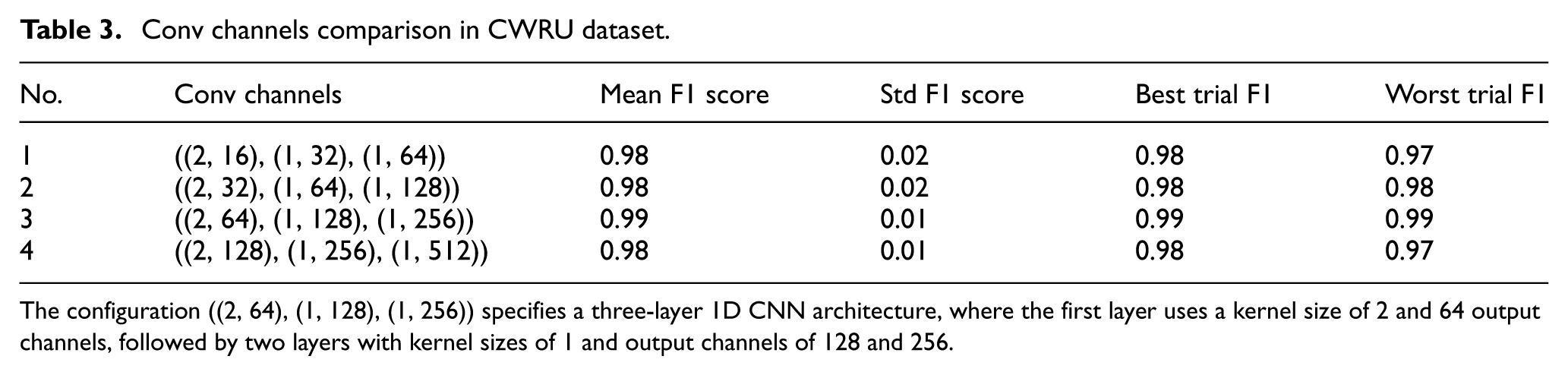
The configuration ((2, 64), (1, 128), (1, 256)) specifies a three-layer 1D CNN architecture, where the first layer uses a kernel size of 2 and 64 output channels, followed by two layers with kernel sizes of 1 and output channels of 128 and 256.

Table 4.

Hidden dimension comparison in CWRU dataset.

No.	Hidden dimension	Mean F1 score	Std F1 score	Best trial F1	Worst trial F1
1	64	0.98	0.02	0.98	0.97
2	128	0.98	0.02	0.98	0.98
3	256	0.99	0.01	0.99	0.99
4	512	0.98	0.01	0.98	0.97
5	1024	0.98	0.01	0.98	0.98

Table 5.

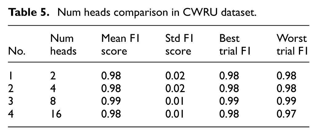
Num heads comparison in CWRU dataset.

No.	Num heads	Mean F1 score	Std F1 score	Best trial F1	Worst trial F1
1	2	0.98	0.02	0.98	0.98
2	4	0.98	0.02	0.98	0.98
3	8	0.99	0.01	0.99	0.99
4	16	0.98	0.01	0.98	0.97

Table 6.

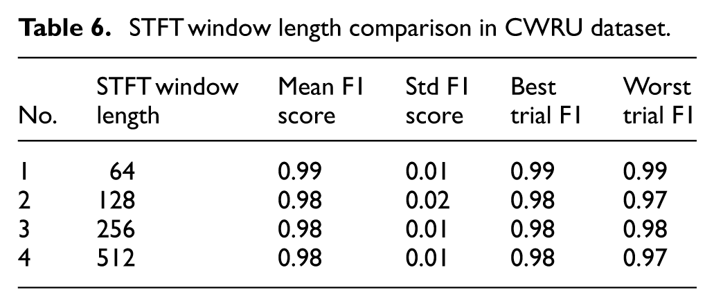
STFT window length comparison in CWRU dataset.

No.	STFT window length	Mean F1 score	Std F1 score	Best trial F1	Worst trial F1
1	64	0.99	0.01	0.99	0.99
2	128	0.98	0.02	0.98	0.97
3	256	0.98	0.01	0.98	0.98
4	512	0.98	0.01	0.98	0.97

Table 7.

Batch size comparison in CWRU dataset.

No.	Batch size	Mean F1 score	Std F1 score	Best trial F1	Worst trial F1
1	8	0.98	0.01	0.99	0.98
2	16	0.99	0.01	0.99	0.99
3	32	0.98	0.01	0.98	0.98
4	64	0.98	0.01	0.98	0.98
5	128	0.98	0.02	0.98	0.98
6	256	0.98	0.01	0.98	0.98

Table 8.

Transformer layers comparison in CWRU dataset.

No.	Transformer layers	Mean F1 score	Std F1 score	Best trial F1	Worst trial F1
1	2	0.98	0.01	0.98	0.98
2	4	0.99	0.01	0.99	0.99
3	6	0.98	0.01	0.98	0.98
4	8	0.98	0.01	0.98	0.98

Table 9.

Hyperparameters setting in CWRU dataset.

Hyperparameter name	Hyperparameter value
Learning rate	0.0001
1D convolutional layer	(2, 64), (1, 128), (1, 256)
Hidden layer size	256
Num of heads	8
Window length of STFT	64
Batch size	16
Num of layers	4

The configuration ((2, 64), (1, 128), (1, 256)) specifies a three-layer 1D CNN architecture, where the first layer uses a kernel size of 2 and 64 output channels, followed by two layers with kernel sizes of 1 and output channels of 128 and 256.

Table 10.

Comparison results in CWRU dataset.

Methods	Accuracy	Precision	Recall	F1-score	AUC
XGBoost 29	89.20	90.42	88.16	88.31	99.21
CNN 29	94.33	94.81	94.33	94.32	99.58
LSTM 29	91.46	91.44	91.44	91.48	99.06
CNN-LSTM 29	96.12	96.12	96.12	96.14	99.64
DEDCNN 28	94.75	94.76	94.78	94.76	99.60
EDAEs 25	94.19	99.20	92.44	92.19	96.48
Swin(CWT) 29	99.22	99.27	99.21	99.21	99.98
MC-CNN 26	99.40	99.48	99.40	99.48	99.98
MMEDL 27	99.70	99.72	99.82	99.91	99.98
RCDAE 29	99.90	99.99	99.99	99.99	99.99
Ours	99.99	99.99	99.99	99.99	99.99

Results

In this study, the proposed model was first trained on the training set and optimized using the validation set, with the hyperparameters yielding the best performance retained. The final model was then rigorously evaluated on the test set. The corresponding confusion matrix and area under the curve, shown in Figures 9 and 10, illustrates the diagnostic results. The model achieved a prediction accuracy of 99.99%.

Figure 9.

Confusion matrix of the proposed model on CWRU dataset.

Figure 10.

Area under the curve of the proposed model on CWRU dataset.

The t-SNE technique was employed to visualize the distribution of classification results based on the optimal base-learner features. The resulting visualization demonstrates that fault categories under different load conditions are effectively separable, indicating well-defined classification boundaries in the feature space. As shown in the t-SNE plot of the diagnostic results, the proposed model exhibits strong classification performance, with clear and distinct boundaries among the 10 fault types (Figure 11).

Figure 11.

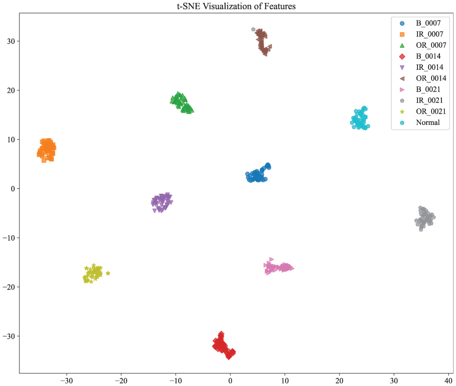
CNN-transformer fault diagnosis model visualization results.

To evaluate the diagnostic capability of the proposed model, its performance was compared against 10 existing methods: XGBoost, CNN, LSTM, CNN-LSTM, EDAEs, Swin Transformer with CWT (Swin(CWT)), MC-CNN, MMEDL, DEDCNN, and RCDAE. XGBoost, ³⁰ an ensemble method, utilizes gradient-boosted decision trees for classification. The baseline CNN model ³⁰ incorporates 3 × 3 convolutional kernels and max-pooling layers. The LSTM model ³⁰ consists of a single LSTM layer with 32 units, followed by a dense Softmax layer. EDAEs ²⁶ represents an ensemble of 15 denoising autoencoders with varied activation functions. The Swin Transformer ³⁰ was implemented using standard module configurations. CNN-LSTM ³⁰ integrates CNN and LSTM structures into a unified diagnostic framework. MC-CNN ²⁷ applies multi-scale 1D convolutions to alleviate local optima issues. MMEDL ²⁸ ensembles various 1D deep CNNs, transforms the extracted features into 2D images, and processes them using a 2D DCNN. DEDCNN ²⁹ is a deep ensemble dense CNN that incorporates AdaBoost for sample weighting. RCDAE ³⁰ is a hybrid ensemble combining Swin Transformer, CNN, and BiLSTM.

All experiments were conducted under the 2 HP load condition of the CWRU dataset. Each method underwent parameter tuning and was evaluated over five independent runs to ensure consistency. The comparison results are presented in Figures 12 to 16 and Table 10. The proposed model achieved average values of 99.99% for accuracy, precision, recall, F1 score, and AUC, outperforming all baseline methods.

Figure 12.

Accuracy comparison of different models on the CWRU dataset.

Figure 13.

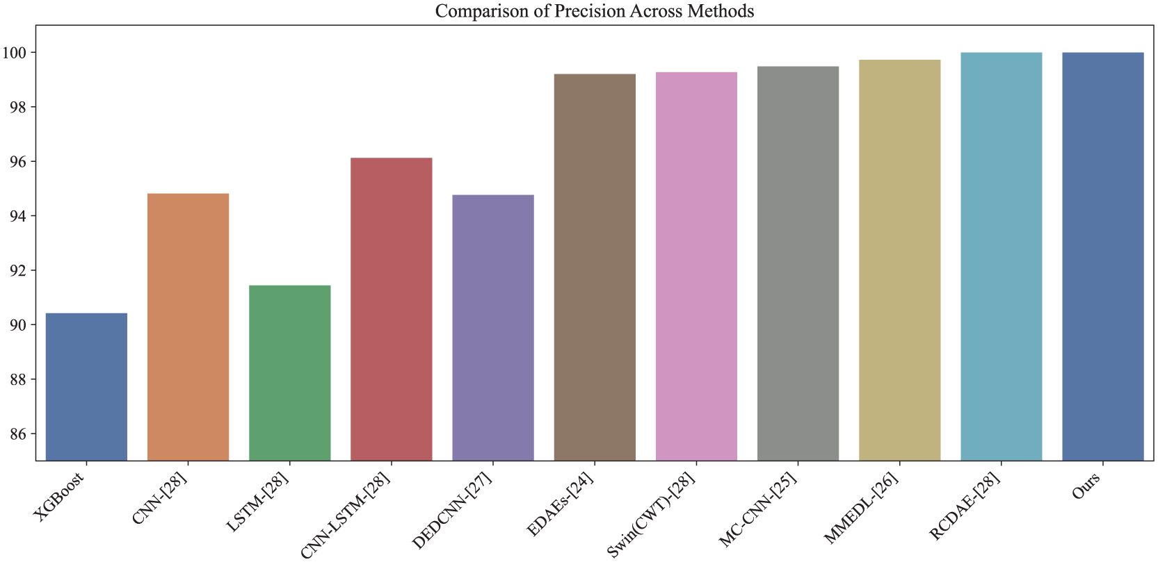
Precision comparison of different models on the CWRU dataset.

Figure 14.

Recall comparison of different models on the CWRU dataset.

Figure 15.

F1-score comparison of different models on the CWRU dataset.

Figure 16.

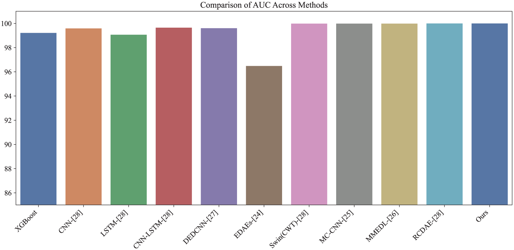
AUC comparison of different models on the CWRU dataset.

To further validate the generalization capability of the proposed model under varying operating conditions and harsh industrial environments, the XJTU-SY bearing dataset was introduced for cross-dataset evaluation. In addition, two ablation variants were designed to assess the necessity of time–frequency feature fusion: Variant A, retaining only the frequency-domain branch, and Variant B, retaining only the time-domain branch.

Under baseline (clean) conditions, both the complete architecture and its ablated variants achieved excellent classification performance, indicating that each individual feature domain is sufficiently discriminative in laboratory environments. However, a clear difference was observed in the convergence behavior. The complete model converged within only 8 training epochs and triggered the early-stopping criterion, whereas Variant B (time-domain only) required up to 29 epochs to reach convergence. This observation aligns with the physical nature of fault signatures: while time-domain features provide raw shock information, they are often overwhelmed by background noise, making optimization difficult. The inclusion of the frequency-domain branch provides a structured spectral template that helps the model “anchor” the fault-related components, thereby significantly accelerating convergence and enhancing diagnostic stability. This result suggests that the joint utilization of time- and frequency-domain features effectively reduces the optimization difficulty of the Transformer encoder. By providing complementary physical representations, the fused input guides the model to rapidly identify discriminative patterns in a higher-dimensional feature space. Beyond convergence efficiency, the diagnostic superiority of the proposed framework is further validated by a quantitative comparison on the XJTU-SY dataset, as summarized in Table 11. In this more challenging task, standard single-domain architectures such as CNN and ResNet only achieved accuracies of 84.3% and 85.0%, respectively, as they struggled to capture the complex non-stationary fault signatures. In contrast, the proposed model reached a near-perfect accuracy of 100% and triggered the early-stopping criterion at only the seventh epoch (see training logs). While the MKPCA + DCResNet method also achieves 100% accuracy, it entails significantly higher computational overhead with 42.51G FLOPs and 17.74M parameters. Our proposed architecture achieves identical precision but with a more streamlined parameter count and lower resource consumption, as discussed in the efficiency analysis. This performance gap demonstrates that the parallel dual-domain strategy is more effective than traditional deep learning models in extracting discriminative features from industrial vibration signals.

Table 11.

Performance and computational complexity comparison on the XJTU-SY dataset.

Method	Accuracy	Precision	Recall	F1-score	AUC
CNN 30	84.30	84.52	84.15	84.33	92.45
ResNet-1830	85.00	85.41	84.78	85.09	94.12
Proposed	99.99	99.99	99.99	99.99	99.99

To further investigate the effectiveness of feature fusion strategies and encoding mechanisms, additive white Gaussian noise (AWGN) was injected into the input signals to simulate complex industrial interference. Special attention was paid to the model performance under extreme noise conditions (−4 dB SNR). The experimental results (see Table 12) demonstrate that the fusion stage plays a critical role in noise robustness. Compared with the late-fusion strategy, which integrates features only at the decision level (accuracy of 45.05%), the early-fusion strategy exhibits a clear advantage, achieving a maximum accuracy of 53.58%. It is noteworthy that although the absolute accuracy under −4 dB SNR is lower than that under clean conditions, it remains significantly higher than the theoretical random guess probability for a 10-class diagnostic task (10%). Given that the noise power at −4 dB is approximately 2.5 times the signal power, the 8.53% improvement over the late-fusion baseline underscores the superior noise-suppression and feature recalibration capabilities of the proposed architecture.

Table 12.

Comparison of fusion and encoding under extreme noise (−4 dB SNR).

Configuration	Accuracy	F1-score	AUC
Late fusion (PE only)	45.05	37.96	76.31
Early fusion (Proposed, None)	53.58	48.81	73.27
Early fusion (PE only)	47.53	40.92	79.05
Early fusion (PE + ME)	43.87	31.69	72.73

From an architectural perspective, early fusion enables the self-attention mechanism of the Transformer to establish global cross-modal interactions between time-domain impulsive characteristics and frequency-domain harmonic components at the feature extraction stage. Under severe noise contamination, the self-attention mechanism can leverage relatively stable frequency distribution patterns to compensate for noise-corrupted time-domain transients, thereby achieving joint correction through multi-source information. In contrast, late fusion lacks such low-level complementary modeling and consequently struggles to extract effective discriminative information when the signal-to-noise ratio is extremely low.

Furthermore, the effects of positional encoding (PE) and modality encoding (ME) on feature representation were systematically analyzed. The results indicate that although introducing positional encoding slightly degrades raw classification accuracy under very low SNR conditions, it significantly enhances prediction confidence. Specifically, the area under the receiver operating characteristic curve (AUC) increased from 0.7327 to 0.7905 after incorporating positional encoding. Interestingly, the inclusion of PE leads to a slight decrease in top-1 accuracy under extreme noise but a substantial gain in AUC. This phenomenon suggests that while intense noise can cause jitter near the decision boundary, the positional awareness provided by PE helps the Transformer maintain a more reliable ranking of potential fault categories, thereby enhancing the overall statistical confidence of the diagnostic system. This improvement suggests that positional encoding endows the model with essential temporal awareness, enabling it to capture the evolutionary patterns of non-stationary vibration signals. Modality encoding, on the other hand, injects explicit modality bias into the feature space, guiding the model to recognize the physical origin of different feature types while mitigating conflicts caused by cross-domain feature heterogeneity.

From the perspective of computational efficiency and practical deployment, the proposed architecture achieves a favorable balance between performance and complexity. Despite incorporating dual-branch feature extractors and sophisticated interaction mechanisms, the model requires only 69.51 MB of GPU memory, and the average inference time for the complete test set is maintained below 4 s. This combination of low resource consumption and efficient inference ensures that the model can be readily deployed on resource-constrained industrial edge devices, satisfying the stringent requirements of real-time condition monitoring.

In summary, the proposed time–frequency fusion architecture demonstrates clear performance gains under extreme operating conditions, substantial improvements in prediction confidence, and efficient convergence behavior. These results provide strong empirical evidence for the “parallel dual-domain” strategy proposed in Section “Introduction,” confirming its robustness in preserving domain-specific fault signatures that are typically attenuated in conventional sequential pipelines. These results collectively confirm its robustness and effectiveness in handling complex, non-stationary vibration signals encountered in real-world industrial applications.

Conclusion

In this study, a parallel time–frequency fusion framework based on CNN and Transformer architectures has been proposed for rolling bearing fault diagnosis. By processing raw vibration signals through dual domain-specific branches and performing feature fusion at an early stage, the proposed method effectively captures complementary transient and spectral characteristics while circumventing the information loss typically associated with sequential domain transformation.

Extensive experiments on the CWRU dataset demonstrate that the proposed framework achieves near-perfect diagnostic accuracy, confirming its strong discriminative capability under standard operating conditions. More importantly, cross-dataset validation on the XJTU-SY bearing dataset (characterized by more complex non-stationary dynamics) further verifies the generalization ability of the proposed approach under varying operating conditions. The results show that early fusion significantly improves noise robustness compared with late fusion, particularly under severe noise contamination (−4 dB SNR), highlighting the importance of cross-modal interaction at the feature level.

Ablation studies reveal that the joint utilization of time- and frequency-domain information not only enhances diagnostic performance but also accelerates model convergence (triggering early stopping significantly sooner than single-domain variants), indicating reduced optimization difficulty for the Transformer encoder when complementary physical representations are jointly provided. Furthermore, the investigation of positional and modality encodings suggests that explicit feature encoding can improve prediction confidence, although its effectiveness depends on signal quality and noise conditions.

From an engineering perspective, the proposed framework maintains a favorable balance between diagnostic performance and computational complexity, exhibiting low memory consumption and efficient inference speed, which makes it suitable for deployment on resource-constrained industrial monitoring systems.

Future work will focus on developing adaptive fusion and encoding strategies that dynamically account for noise levels and operating conditions, as well as extending the proposed framework to more diverse industrial scenarios involving variable speeds, loads, and compound fault types.