Sage Journals: Discover world-class research

Abstract

The autonomous vehicle can recognize and understand environment, self-control, and achieve the driving level of the human driver. To create this kind of system, the following work was carried out: (a) a real time lane detection system is proposed, based on vision system functions, using webcam camera; (b) In order to detect curve lanes, deep learning is applied for lane detection, based on fully Convolutional Neural Network (CNN); (c) The cubic spline interpolation method is used for path generation, based on Global Positioning System (GPS) data, where distance between two adjacent path generation points is same. Compared with the connection method of the cubic polynomial fitting algorithm, the curve fitted path by the cubic spline interpolation method is smoother and more satisfied with the vehicle motion pattern; (d) Based on frenet coordinate frame, optimize trajectory planning method is used to plan safe, easy and comfort trajectory. Compared to the Cartesian coordinate frame, frenet coordinate frame simplifies the solution of road curve fitting problems, especially in the case of complex road environment; (e) Fuzzy sliding mode control method is proposed for vehicle steering control. Finally, the simulation and experiment results are used to prove the effectiveness of the proposed methods.

Keywords

Autonomous vehicle system real time lane detection lane detection using fully CNN path generation trajectory planning fuzzy sliding mode control method for steering control

Introduction

Autonomous vehicle systems have been a popular topic of research. The technical preparation of self-driving vehicles is maturing, with the increase in available computing power and the reduction in sensor costs.¹ The field of self-driving technology is not only related to vehicle control, path planning, sensory fusion, but also forewords such as artificial intelligence, machine learning, deep learning, and reinforcement learning. Self-driving will start a new technology and market revolution, in the next 5 to 10 years. Autonomous driving has been of interest to researches to push the boundaries of automotive racking, that is limited by the abilities of human drivers, with several companies and academics. Stanford University developed an off-road autonomous vehicle for the DARPA Grand Challenge.² Hanyang University developed an autonomous off-road Hyundai “A1” to compete in the Autonomous Vehicle Competition (AVC).³ Google has tested its self-driving vehicles over 2 million miles, using 100 self-driving vehicles.⁴ Tesla provides self-driving function in their 2016 model S cars.⁵ Uber’s plans to eventually replace the human driven fleet with self-driving cars.⁶

The core of the self-driving system, including three parts: perception, planning, and control. Self-driving system technology means that: self-driving car can recognize the surrounding environment and status of the vehicle through a variety of on-board sensors (camera, lidar, millimeter wave radar, GPS, inertial sensors, etc.), and make analysis and judgment, then autonomously control vehicle movement, and finally achieve self-driving based on the acquired environmental information (including road information, traffic information, vehicle location and Obstacle information, etc.) This paper proposes methods for self-driving system in perception, planning and control, based on on-board sensors.

In lane detection and tracking, several issues should be considered, namely choosing an appropriate lane model, developing an image processing for features extraction, probability of lane tracking, and effectiveness of real-time image processing ability.⁷ Based on,⁸ three main methods for lane detection using cameras includes: model of the lane markings, color information, and feature information method including edge, gradient and intensity.^9,10 About road information, it makes the mathematical model of the lane markings, such as B-spline,¹¹ where candidate points are extracted from the lane markings. About color information, it applies a threshold to the image based on RGB and HSL color space, and places an 8-bit image.¹² To extract a lane, color threshold is based on RGB color space or HSL color space. Due to simplification of computer monitor design, the RGB color space is the most commonly used color space. However, it cannot be used for all applications. In order to describe a color in the RGB color space, the red, green, and blue color components are all used, so RGB is not as intuitive as other color spaces. The HSL color space uses only the hue component to describe color. Therefore, HSL is the best color space for image processing applications, for example color matching.¹³ In this paper, a real-time lane detection system is proposed, which uses the capabilities of vision system functions, based on combination of feature information and color information.

The real-time lane detection system works well for clear straight lane. However, on curved lanes or sharp turns, the real time lane detection system would fail, due to complexity of the lane markers. The lane detector cannot distinguish the lane edge well. The lane detection system based on Convolutional Neural Network (CNN) can overcome this problem. CNN is the most popular deep learning architecture, due to the effectiveness of convnets. The main advantage of CNN is that it can automatically detect the important features without any human supervision. CNN is also computationally efficient. This enables CNN models to run on any device.¹⁴

Path planning can be divided into two steps: global path planning and local path planning. Global path planning deals with generating the most ideal route to reach the final destination. Local path planning is responsible for obstruction avoidance and path planning for each segment generated by the global path planner.¹⁵ There are some methods for local path planning, such as artificial potential field method, A* algorithm, and discrete optimization approach. The artificial potential method is calculated by the attractive and repulsive potential functions. However, the computations are complex and sometimes unsolvable, because the path is described in high order polynomial.¹⁶ In addition, it does not always yield a path to the goal due to local minima in the vector field.¹⁷ For A* algorithm, it does not work well on lane tracking based on driving with few obstacles.¹⁷ The discrete optimization approach calculates a finite number of paths. A cost is computed for each path, and finally the path with least cost is selected. In this paper, a discrete optimization method¹⁸ is used, based on the frenet coordinate system for autonomous vehicle path planning, which has strong practicability in assisted driving and self-driving.

Fuzzy logic is widely used in motion control, because it provides the ability to control system with construction of complex mathematical model. Fuzzy logic is used for mobile robot motion control, where sensors of mobile robot contain uncertain and incomplete information.¹⁹ Fuzzy logic technology is also used in traffic management. There is applicability issue to create models of traffic, but IF-THEN logic can deal with vague expectations and respond to situations.²⁰ In this paper, fuzzy sliding mode control method is used to minimize vehicle’s steering angle error. The vehicle’s cross track error is defined as $δ_{iE}$ . An angular velocity control law is designed to make the cross-track error to zero.

The contribution of this paper is: (a) A real time lane detection system is proposed based on vision system functions, where image acquisition and processing functions are used to extract lanes. Although there exists lane detection algorithms in previous work, the proposed lane detection system processes fast and the performance is good. (b) In order to detect curve lanes, deep learning is applied for lane detection, based on fully CNN. It shows how to perform lane segment detection by training a deep neural network for lane segmentation. Compared with,²¹ in this paper, the number of layers is increased, and the number of convolution kernels is modified in each layer. A parallel jump structure is used to connect the encoding feature map to the decoding feature map. UpSampling2D is changed to Conv2D Transpose to implement the upsampling process. (c) The cubic spline interpolation method is used for path generation, based on GPS data, where distance between two adjacent path generation points is same. Compared with the connection method of the cubic polynomial fitting algorithm, the curve fitted path by the cubic spline interpolation method is smoother and more satisfied with the vehicle motion pattern. (d) Optimize trajectory planning method depending on frenet coordinate frame is used to plan the safe, easy and comfort trajectory. In addition, compared to the Cartesian coordinate frame, frenet coordinate frame simplifies the solution of road curve fitting problems, especially in the case of complex road environment. Compared with pure pursuit algorithm, the result shows that the path planned by optimize trajectory planning method is more closed to the predefined path. (e) fuzzy sliding mode control method is used to design angular velocity control law to minimize vehicle’s steering angle error. (f) the simulation and experiment results show effectiveness of the proposed methods.

In this paper, section 2 gives the modeling of the vehicle. Section 3 describes two lane detection systems. Section 4 discusses the path generation and path planning methods. Section 5 outlines the fuzzy sliding mode method for vehicle steering control. Section 6 and Section 7 show the simulation result and experiment result, respectively.

Modeling

The local and global coordinate of the vehicle is shown as Figure 1. $X_{l} M Y_{l}$ is the local coordinate frame. $X_{g} O Y_{g}$ is the global coordinate frame. $M_{r}$ is the central point of rear axle, which is the original point of local coordinate frame. $M_{f}$ is the central point of front axle. The angular difference between the global and local coordinate is given by $θ$ . The orientation of the local coordinate frame about the global coordinate frame is expressed by the rotation matrix as

R (θ) = [\begin{matrix} \cos θ & \sin θ & 0 \\ - \sin θ & \cos θ & 0 \\ 0 & 0 & 1 \end{matrix}]

(1)

Figure 1.

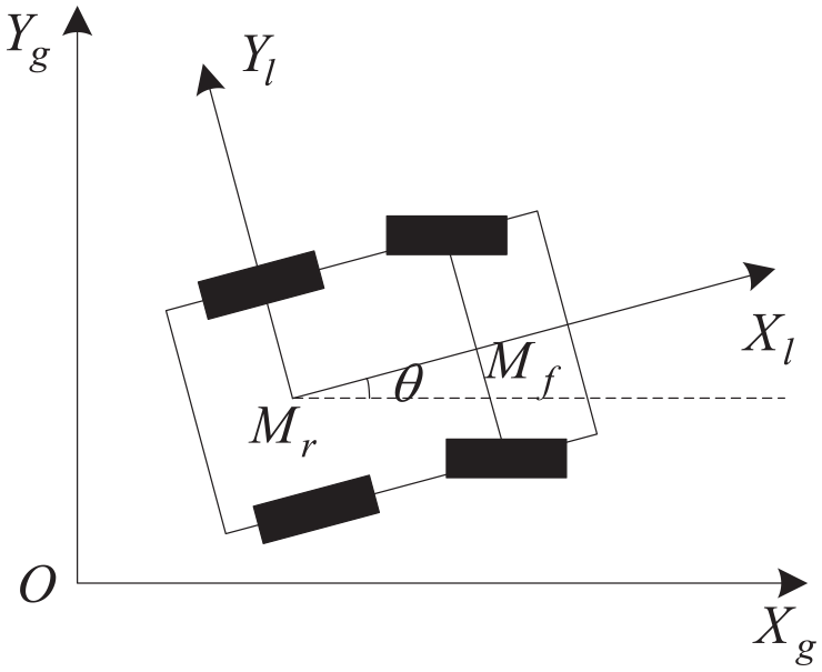
The local and global coordinate of the vehicle.

The local coordinate of the system is shown in Figure 2, where $l$ is the wheelbase, $φ$ is wheel steering angle, $d$ is the distance between two rear wheels, ICR is instantaneous center of rotation, and $d_{r}$ and $d_{f}$ are instantaneous radius of rotation of $M_{r}$ and $M_{f}$ , respectively. The overall speed of the vehicle $v_{r}$ is the speed of rear wheels, along with the axes direction of $X_{l}$ of local coordinate frame. $v_{f}$ is the speed of front wheels. The relationship of $v_{r}$ and $v_{f}$ is:

v_{f} = v_{r} / \cos φ

(2)

Figure 2.

Local coordinate system of the vehicle.

In Figure 3, point w is the center gravity point of the car. The configuration of the vehicle about point W is defined as $[x, y, δ]^{T}$ in global coordinate. $x$ , $y$ and $δ$ are the x coordinate, y coordinate, and orientation of the vehicle, respectively. $v$ is the speed of the vehicle. $w_{f}$ and $w_{r}$ are the distances between the center gravity point and the front wheel and the rear wheel, respectively. The kinematic model of the vehicle is calculated as

[\begin{matrix} \overset{\cdot}{x} \\ \overset{\cdot}{y} \\ \overset{\cdot}{δ} \end{matrix}] = [\begin{matrix} v \cos (δ + β) \\ v \sin (δ + β) \\ \frac{v}{w_{r}} \sin (β) \end{matrix}]

(3)

where $β$ is calculated as:

β = arc \tan (\frac{w_{r}}{w_{r} + w_{f}} \tan (φ))

(4)

Figure 3.

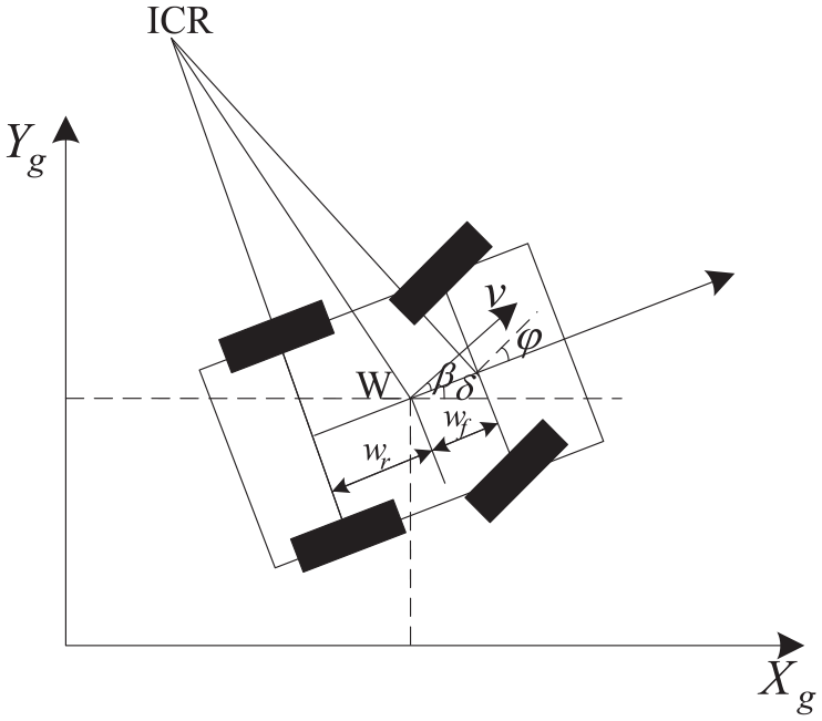
The kinematic model of the vehicle.

Lane detection system

Real time lane detection system

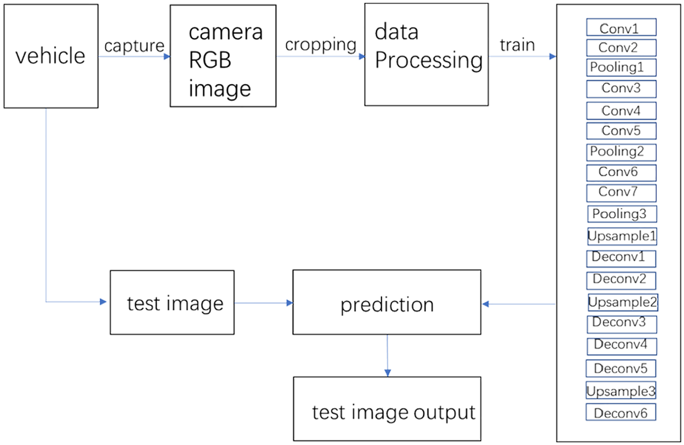
A webcam camera is equipped in front of the vehicle. Using the camera, the vehicle detects lane, and tracks lane. The real time lane detection system flowchart is shown in Figure 4. Firstly, the camera acquires image. In the second block, the image is resized to 640×480 for image processing. Because on the road, there are always two lanes. The lanes are straight or curve. The lanes are also solid lanes or dash lanes. Based on lane characteristics, four rectangle regions of interest (ROI) are defined to focus on lane area and analyze the lane data. Two ROIs are used to focus on left lane, and two ROIs are for the right lane, in order to detect dash and curve lane. Color threshold block coverts a color image to a binary image. If the color components are in the specified range, the pixel value of the original image will be set to 1. Otherwise, the pixel value is equal to 0. The color threshold, based on HSL color space, is used to extract lane. Hue channel is used to detect yellow lane. Luminance channel is for white lane detection. In order to remove or enhance isolated feature, grayscale morphology is used. Two functions are used in this block: erosion and dilation. Erosion reduces the brightness of pixels surrounded by neighbors with a lower intensity. Dilation increases the brightness of pixels, which are surrounded by neighbors with a higher intensity. Based on the environment condition, erosion or dilation is chosen for gray morphology. Finding edge block is used to find a line describing the edge with points along the edge, and output the coordinate information of the points. Converting pixel to real world is applied to transform pixel coordinate to real-world coordinate. For obtaining lane tracking points block, the algorithm is processed as Figure 5. $B_{i} (x_{bi}, y_{bi})$ and $C_{i} (x_{ci}, y_{ci})$ are the edge points coordinates, based on finding edge and converting pixel to real world blocks. The tracking points $A_{i} (x_{ai}, y_{ai})$ is based on its configuration in (3) and (4), and calculated as.

x_{ai} = \frac{1}{2} (x_{bi} + x_{ci})

(5)

y_{ai} = \frac{1}{2} (y_{bi} + y_{ci})

(6)

Figure 4.

Real time lane detection system flowchart.

Figure 5.

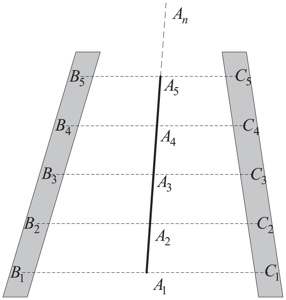
Obtaining lane tracking points.

Lane detection system using fully CNN

In this section, deep learning is applied to detect lanes based on fully CNN. It shows how to perform lane segment detection by training a deep neural network for lane segmentation. SegNet is an encoding-decoding structure. It uses different method in upsampling and downsampling. Based on,²¹ Figure 6 shows pipeline used in lane detection system. The neural network architecture includes seven convolutional layers, three polling layers, three upsampling layer and seven deconvolution layers. However, this model is not stable during lane detection, so the model is improved in this paper as shown in Figure 7. Different from network in Figure 6, the number of layers is increased in the network. The number of convolution kernels is modified in each layer. A parallel jump structure is used to connect the encoding feature map to the decoding feature map, so that multi-layer information can be used in classification prediction. UpSampling2D is changed to Conv2D Transpose to implement the upsampling process, since Conv2DTranspose has the process of learning, which has better result. The BDD100K data is used, consisting of images and labels. For training, the dataset is divided into training set and validation set. The neural network architecture includes 10 convolutional layers, four polling layers, four concatenate layers and 10 deconvolution layers. The model is compiled with mean squared error as the loss function. And the model is trained on the training set, and validated on the validation dataset. Images are inputs of prediction process. Using the trained model result, the prediction process outputs images with regions of the detected lane.

Figure 6.

Pipeline used in lane detection system.²¹

Figure 7.

Pipeline used in lane detection system for this paper.

Path generation and path planning

Cubic spline interpolation model

Autonomous vehicles do path planning and tracking algorithm based on GPS data. However, due to communication delay, the GPS data cannot be obtained continuously. Distances between each two conjunction GPS points are not same. Therefore, if the GPS data is directly used to do the path planning and tracking algorithm, without path generation algorithm, the speed of the vehicle is always changed. In order to control autonomous vehicle smoothly and safely movement, constant speed is pursued for the vehicle. The cubic spline interpolation method is used for path generation, based on GPS data, where distances between two adjacent path generation points are the same. Compared with the connection method of the cubic polynomial fitting algorithm, the curve fitted path by the cubic spline interpolation method is smoother and more satisfied with the vehicle motion pattern. The cubic polynomial fitting algorithm produces a curve arc in some straight lines’ segments. This is not the expected vehicle operating characteristic. Based on vehicle kinematics, the vehicle should take a straight line as much as possible. Only in the direction of the transition, a curved path, which matches the vehicle turning characteristics, is needed. The feature of cubic spline interpolation method is as:

The cubic spline curve is continuous and smooth at the joint.

The first and second derivatives of the cubic spline are continuous.

The second derivative of the boundary of the natural cubic spline is continuous.

A single point does not affect the entire interpolation curve.

Three points $S_{1} = (x_{1}, y_{1})$ , $S_{2} = (x_{2}, y_{2})$ , and $S_{3} = (x_{3}, y_{3})$ are defined to be fitted. The cubic functions to fit points $S_{1}$ and $S_{2}$ , to fit points $S_{2}$ and $S_{3}$ are calculated as

y = a x^{3} + b x^{2} + cx + d

(7)

y = e x^{3} + f x^{2} + gx + h

(8)

Equation (7) passes through $S_{1}$ and $S_{2}$ , and equation (8) passes through $S_{2}$ and $S_{3}$ , so the following equations can be obtained:

y_{1} = {ax}_{1}^{3} + {bx}_{1}^{2} + c x_{1} + d

(9)

y_{3} = {ex}_{1}^{3} + {fx}_{1}^{2} + g x_{1} + h

(10)

{ax}_{2}^{3} + {bx}_{2}^{2} + c x_{2} + d = e x_{2}^{3} + {fx}_{2}^{2} + g x_{2} + h = y_{2}

(11)

Based on feature 2, the first derivative of both sides of equation (11) can be obtained as:

3 {ax}_{2}^{2} + 2 b x_{2} + c x_{2} = 3 e x_{2}^{2} + 2 f x_{2} + g

(12)

Based on feature 3, the second derivative at the start and end points should be continuous, the following are obtained.

6 a x_{1} + 2 b = 0

(13)

6 e x_{3} + 2 f = 0

(14)

Supposed that there are n+1 path points: $(x_{0}, y_{0})$ , $(x_{1}, y_{1})$ , $(x_{2}, y_{2})$ , …, $(x_{n}, y_{n})$ . The difference between two conjunction points is calculated as

h_{i} = x_{i + 1} - x_{i}, i = 0, 1, . . ., n + 1

(15)

Combining the above six equations (9) to (14), the parameters $a, b, c, d$ in the cubic spline interpolation function can be calculated.

a_{i} = y_{i}

(16)

b_{i} = \frac{y_{i + 1} - y_{i}}{h_{i}} - \frac{h_{i}}{2} m_{i} - \frac{h_{i}}{6} (m_{i + 1} - m_{i})

(17)

c_{i} = \frac{m_{i}}{2}

(18)

d_{i} = \frac{m_{i + 1} - m_{i}}{6 h_{i}}

(19)

where $m_{i}$ is the solution of the following matrix equation.

[\begin{matrix} 1 & 0 & 0 & 0 & \dots & 0 \\ h_{0} & 2 (h_{0} + h_{1}) & h_{1} & 0 & 0 & 0 \\ 0 & h_{1} & 2 (h_{1} + h_{2}) & h_{2} & 0 & 0 \\ 0 & 0 & h_{2} & 2 (h_{2} + h_{3}) & h_{3} & ⋮ \\ ⋮ & 0 & 0 & ⋱ & ⋱ & ⋱ \\ 0 & 0 & 0 & h_{n - 2} & 2 (h_{n - 2} + h_{n - 1}) & h_{n - 1} \\ 0 & \dots & 0 & 0 & 0 & 1 \end{matrix}] [\begin{matrix} m_{0} \\ m_{1} \\ m_{2} \\ m_{3} \\ ⋮ \\ m_{n} \end{matrix}] = 6 [\begin{matrix} 0 \\ \frac{y_{2} - y_{1}}{h_{1}} - \frac{y_{1} - y_{0}}{h_{0}} \\ \frac{y_{3} - y_{2}}{h_{2}} - \frac{y_{2} - y_{1}}{h_{1}} \\ \frac{y_{4} - y_{3}}{h_{3}} - \frac{y_{3} - y_{2}}{h_{2}} \\ ⋮ \\ \frac{y_{n} - y_{n - 1}}{h_{n - 1}} - \frac{y_{n - 1} - y_{n - 2}}{h_{n - 2}} \\ 0 \end{matrix}]

(20)

Optimization of trajectory planning method based on frenet coordinate frame

Frenet coordinate frame

The centerline of the road is defined as the road reference line. As shown in Figure 8, a frenet coordinate frame is established using the tangent vector t of the reference line and the normal vector n. The coordinate frame is based on the starting road center line, and the coordinate axes are perpendicular to each other. The direction of the road reference line is $s$ direction, which is called longitudinal direction. The normal direction of the reference line is $d$ direction, which is called lateral direction. Compared to the Cartesian coordinate frame, frenet coordinate frame simplifies the solution of road curve fitting problems, especially in the case of complex road environment, since it is easy to find the road reference line and describe the location of the vehicle, based on the longitudinal direction and lateral direction. Compared with the Cartesian coordinate system, the frenet coordinate system simplifies the solution of the road curve fitting problem. In the road environment, we can always find the reference line of the road, which is the center line of the road. Therefore, the vehicle position, based on the reference line, can be simply represented using the distance along the longitudinal direction and the distance along the lateral direction. The calculation of the speed in both directions is also relatively simple, based on frenet coordinate system.

Figure 8.

Frenet coordinate frame.

Optimization trajectory planning method

Due to lane change or obstacle avoidance, there is a certain lateral offset between the car and the desired lane. The car should return to its desired lane, based on the best compromise result between the comfort experience in the car and the time required to reach the desired lane position. In longitudinal direction, if the car is moving too fast or too close to the front car, it must slow down significantly without rushing. Comfort can be described by the jerk, which is difference of acceleration.¹⁸ Based on,²² a quantic polynomial is the jerk-optimal connection of a start state $P_{0} = [p_{0}, {\overset{\cdot}{p}}_{0}, {\overset{\cdot\cdot}{p}}_{0}]$ and an end state $P_{1} = [p_{1}, {\overset{\cdot}{p}}_{1}, {\overset{\cdot\cdot}{p}}_{1}]$ within the time interval $T = t_{1} - t_{0}$ in a one-dimensional problem. The jerk can be described as:

J_{t} (p (t)) = \int_{t_{0}}^{t_{1}} {\overset{\dots}{p}}^{2} (τ) d τ

(21)

where $p (t)$ is described as:

p (t) = α_{0} + α_{1} t + α_{2} t^{2} + α_{3} t^{3} + α_{4} t^{4} + α_{5} t^{5}

(22)

Trajectory plan in lateral direction

In Lateral Direction, define the start state as $D_{0} = [d_{0}, {\overset{\cdot}{d}}_{0}, {\overset{\cdot\cdot}{d}}_{0}]$ , based on equation (22), the lateral offset, lateral velocity, and lateral acceleration of the start state are described as

\begin{matrix} d_{0} = d (t_{0}) = α_{d 0} + α_{d 1} t_{0} + α_{d 2} t_{0}^{2} \\ + α_{d 3} t_{0}^{3} + α_{d 4} t_{0}^{4} + α_{d 5} t_{0}^{5} \end{matrix}

(23)

{\overset{\cdot}{d}}_{0} = \overset{\cdot}{d} (t_{0}) = α_{d 1} + 2 α_{d 2} t_{0} + 3 α_{d 3} t_{0}^{2} + 4 α_{d 4} t_{0}^{3} + 5 α_{d 5} t_{0}^{4}

(24)

{\overset{\cdot\cdot}{d}}_{0} = \overset{\cdot\cdot}{d} (t_{0}) = 2 α_{d 2} + 6 α_{d 3} t_{0} + 12 α_{d 4} t_{0}^{2} + 20 α_{d 5} t_{0}^{3}

(25)

Define the end state as $D_{1} = [d (t_{1}), \overset{\cdot}{d} (t_{1}), \overset{\cdot\cdot}{d} (t_{1})]$ , the lateral offset, lateral velocity, and lateral acceleration of the end state are described as

\begin{matrix} d_{1} = d (t_{1}) = α_{d 0} + α_{d 1} t_{1} + α_{d 2} t_{1}^{2} \\ + α_{d 3} t_{1}^{3} + α_{d 4} t_{1}^{4} + α_{d 5} t_{1}^{5} \end{matrix}

(26)

{\overset{\cdot}{d}}_{1} = \overset{\cdot}{d} (t_{1}) = α_{d 1} + 2 α_{d 2} t_{1} + 3 α_{d 3} t_{1}^{2} + 4 α_{d 4} t_{1}^{3} + 5 α_{d 5} t_{1}^{4}

(27)

{\overset{\cdot\cdot}{d}}_{1} = \overset{\cdot\cdot}{d} (t_{1}) = 2 α_{d 2} + 6 α_{d 3} t_{1} + 12 α_{d 4} t_{1}^{2} + 20 α_{d 5} t_{1}^{3}

(28)

Define $t_{0} = 0$ , $α_{d 0}$ , $α_{d 1}$ , and $α_{d 2}$ are calculated as

α_{d 0} = d (t_{0})

(29)

α_{d 1} = \overset{\cdot}{d} (t_{0})

(30)

α_{d 2} = \frac{\overset{\cdot\cdot}{d} (t_{0})}{2}

(31)

$α_{d 3}$ , $α_{d 4}$ , and $α_{d 5}$ can be calculated based on the following matrix

\begin{matrix} [\begin{matrix} α_{d 3} \\ α_{d 4} \\ α_{d 5} \end{matrix}] = {[\begin{matrix} T^{3} & T^{4} & T^{5} \\ 3 T^{2} & 4 T^{3} & 5 T^{4} \\ 6 T & 12 T^{2} & 20 T^{3} \end{matrix}]}^{- 1} \\ [\begin{matrix} d (t_{1}) - (d (t_{0}) + \overset{\cdot}{d} (t_{0}) T + \frac{1}{2} \overset{\cdot\cdot}{d} (t_{0}) T^{2}) \\ \overset{\cdot}{d} (t_{1}) - (\overset{\cdot}{d} (t_{0}) + \overset{\cdot\cdot}{d} (t_{0}) T) \\ \overset{\cdot\cdot}{d} (t_{1}) - \overset{\cdot\cdot}{d} (t_{0}) \end{matrix}] \end{matrix}

(32)

Instead of calculating the best trajectory, a series of candidate trajectories are generated, and then a valid trajectory with the least cost path is selected. The cost function is described as:

C_{d} = k_{j} J_{t} (d (t)) + k_{t} T + k_{d} d_{1}^{2}

(33)

where $k_{j}$ , $k_{t}$ , $k_{d} > 0$ . Item $k_{j} J_{t} (d (t))$ is used to penalize the candidate trajectory with higher Jerk. Item $k_{t} T$ represents the breaking time. Item $k_{d} d_{1}^{2}$ describes the difference between the goal state with the reference line. For the optimizing trajectory, the vehicle should move in parallel to the center line, so $d_{1}$ is a constant and ${\overset{\cdot}{d}}_{1} = {\overset{\cdot\cdot}{d}}_{1} = 0$ . Combining different end conditions $d_{i} \in (d_{\min}, d_{\max})$ and $T_{j} \in (T_{\min}, T_{\max})$ , the candidate trajectories can be calculated as

[d_{1}, {\overset{\cdot}{d}}_{1}, {\overset{\cdot\cdot}{d}}_{1}, T]_{ij} = [d_{i}, 0, 0, T_{j}]

(34)

where $d_{\min}$ , $d_{\max}$ and $T_{\min}$ , $T_{\max}$ are the constraints for $d_{i}$ and $T_{j}$ , respectively. Define $Δ d$ and $Δ T$ as sampling density, equations (35) and (36) can be described as:

d_{i + 1} = d_{i} + Δ d

(35)

T_{j + 1} = T_{j} + Δ T

(36)

Trajectory plan in longitudinal direction

In order to plan trajectory in longitudinal direction, three conditions are considered: following, merging and stopping, and keeping at a constant speed. To calculate the cost function, for the following, merging and stopping cases, the start state is set as $S_{0} = [s_{0}, {\overset{\cdot}{s}}_{0}, {\overset{\cdot\cdot}{s}}_{0}]$ , and the target position $s_{target}$ is defined. For the velocity keeping case, the target velocity ${\overset{\cdot}{s}}_{target}$ is defined.

For the following cases, the target position is defined as:

s_{target} (t) = s_{lv} (t) - [D_{0} + τ {\overset{\cdot}{s}}_{lv} (t)]

(37)

where $D_{0}$ and $τ$ are constants. $s_{lv}$ and ${\overset{\cdot}{s}}_{lv}$ are the position and velocity of the leader vehicle, which are described as below, with assumption ${\overset{\cdot\cdot}{s}}_{l v} (t) = {\overset{\cdot\cdot}{s}}_{l v} (t_{0}) = c o n s t$ .

{\overset{\cdot}{s}}_{lv} (t) = {\overset{\cdot}{s}}_{lv} (t_{0}) + {\overset{\cdot\cdot}{s}}_{lv} (t_{0}) [t - t_{0}]

(38)

s_{lv} (t) = s_{lv} (t_{0}) + {\overset{\cdot}{s}}_{lv} (t_{0}) [t - t_{0}] + \frac{1}{2} {\overset{\cdot\cdot}{s}}_{lv} (t_{0}) [t - t_{0}]^{2}

(39)

The first derivative and second derivative of $s_{target} (t)$ are given as

{\overset{\cdot}{s}}_{target} (t) = {\overset{\cdot}{s}}_{lv} (t) - τ {\overset{\cdot\cdot}{s}}_{lv} (t)

(40)

{\overset{\cdot\cdot}{s}}_{target} (t) = {\overset{\cdot\cdot}{s}}_{lv} (t_{1}) - τ {\overset{\dots}{s}}_{lv} (t) = {\overset{\cdot\cdot}{s}}_{lv} (t_{1})

(41)

For merging case, the target position is defined as:

s_{target} (t) = \frac{1}{2} [s_{a} (t) + s_{b} (t)]

(42)

where $s_{a} (t)$ and $s_{b} (t)$ are pair of vehicles’ positions, which the vehicle should merge.

For stopping case, the target position is defined as:

s_{target} (t) = s_{stop} (t)

(43)

where ${\overset{\cdot}{s}}_{stop} = {\overset{\cdot\cdot}{s}}_{stop} = 0$ . Combining different end conditions $Δ s_{i}$ and $T_{j}$ as below, candidate trajectories can be computed.

[s_{1}, {\overset{\cdot}{s}}_{1}, {\overset{\cdot\cdot}{s}}_{1}, T]_{ij} = [[s_{target} T_{j} + s_{i}], {\overset{\cdot}{s}}_{target} T_{j}, {\overset{\cdot\cdot}{s}}_{target} T_{j}, T_{j}]

(44)

For these two cases, the cost function is expressed as:

C_{s} = k_{j} J_{t} (s (t)) + k_{t} T + k_{s} [s_{1} - s_{target}]^{2}

(45)

In the keeping at a constant speed case, for a start state $S_{0} = [s_{0}, {\overset{\cdot}{s}}_{0}, {\overset{\cdot\cdot}{s}}_{0}]$ and an end state $S_{1} = [{\overset{\cdot}{s}}_{1}, {\overset{\cdot\cdot}{s}}_{1}]$ , combining different end conditions $Δ s_{i}$ and $T_{j}$ as below, candidate trajectories can be computed.

[{\overset{\cdot}{s}}_{1}, {\overset{\cdot\cdot}{s}}_{1}, T]_{ij} = [[{\overset{\cdot}{s}}_{target} T_{j} + Δ {\overset{\cdot}{s}}_{i}], 0, T_{j}]

(46)

The cost function is expressed as:

C_{s} = k_{j} J_{t} (s (t)) + k_{t} T + k_{s} [Δ {\overset{\cdot}{s}}_{1} - {\overset{\cdot}{s}}_{target}]^{2}

(47)

Finally, comparing the cost function in lateral direction and the cost function in longitudinal direction as below, the best trajectory can be selected.

C_{total} = k_{lat} C_{d} + k_{lon} C_{s}

(48)

where $k_{lat}$ and $k_{lon}$ are the constants. $C_{d}$ and $C_{s}$ are the cost function in lateral direction and in longitudinal direction. The trajectory, which has the minimize value of $C_{total}$ , is the optimization trajectory.

Fuzzy sliding control method for vehicle steering

The vehicle movement along a predefined trajectory is expected in constant speed. If constant steering angle is used to control the vehicle, the vehicle’s movement will be oscillatory. For solving the problem, we propose a fuzzy sliding mode control method to control vehicle’s steering angle. Define the vehicle’s cross track error as $δ_{iE}$ . The switching function $s_{i}$ is as:

s_{i} = δ_{iE}

(49)

The exponential reaching law is designed as

{\overset{\cdot}{s}}_{i} = - k_{1} sgn s_{i} - k_{2} s_{i}

(50)

where $k_{1} > 0$ , $k_{2} > 0$ , $sgn s_{i} = \frac{s_{i}}{| s_{i} | + σ}$ , $σ$ is a positive constant.

The control law is defined as

ω_{i} = ω_{iw} + k_{1} sgn s_{i} + k_{2} s_{i}

(51)

In order to prove the stability of the control law, the Lyapunov function is designed as

V_{i} = \frac{1}{2} δ_{iE}^{2}

(52)

The derivative of the Lyapunov function is

{\overset{\cdot}{V}}_{i} = θ_{iE} {\overset{\cdot}{θ}}_{iE} = s \overset{\cdot}{s} = - k_{1} | s_{i} | - k_{2} s_{i}^{2} \leq 0

(53)

When $δ_{iE} = 0$ , $\overset{\cdot}{V} = 0$ . When $θ_{iE} \neq 0$ , ${\overset{\cdot}{V}}_{i} < 0$ . Therefore, the system is asymptotically stable.

$k_{1}$ should be large to have fast trending motion from system status to sliding surface, if a moving point is far from the sliding surface. Otherwise, $k_{1}$ should be small to have slow trending motion to weaken the charting. Therefore, the fuzzy sliding mode controller is designed, where the fuzzy rule is described as Table 1. Seven fuzzy variables are used to describe the fuzzy partitions, as positive big (PB), positive medium (PM), positive small (PS), zero (ZO), negative small (NS), negative medium (NM), negative big (NB).

Table 1.

Fuzzy rule.

$\| \bar{S} i \|$	PB	PM	PS	ZO	NS	NM	NB
${\bar{k}}_{1}$	PB	PM	PS	ZO	NS	NM	NB
${\bar{k}}_{2}$	NB	NM	NS	ZO	PS	PM	PB

The triangular function is defined as:

f (x) = {\begin{matrix} max (0, 1 - \frac{2 (a - x)}{w}), x \leq a \\ max (0, 1 - \frac{2 (x - a)}{w}), x > a \end{matrix}

(54)

The output is based on centroid defuzzification method, and is given as (55). $μ ({\bar{k}}_{1})$ and $μ ({\bar{k}}_{2})$ are the membership value for point ${\bar{k}}_{1}$ and point ${\bar{k}}_{2}$ , respectively.

{\bar{k}}_{1} = \frac{\sum_{i = 1}^{7} {\bar{k}}_{1} μ ({\bar{k}}_{1})}{\sum_{i = 1}^{7} μ ({\bar{k}}_{1})}, {\bar{k}}_{2} = \frac{\sum_{i = 1}^{7} {\bar{k}}_{2} μ ({\bar{k}}_{2})}{\sum_{i = 1}^{7} μ ({\bar{k}}_{2})}

(55)

The fuzzy exponential reaching law is defined as

{\overset{\cdot}{s}}_{i} = - {\bar{k}}_{1} sgn s_{i} - {\bar{k}}_{2} s_{i}

(56)

The fuzzy sliding mode control law is as

ω_{i} = ω_{iw} + {\bar{k}}_{1} sgn s_{i} + {\bar{k}}_{2} s_{i}

(57)

Simulations

Real time lane detection simulation

The powerful capabilities of LabVIEW are used to simulate lane detection. The original figure is shown in Figure 9. The vehicle should detect yellow lane and white lane, simultaneously. To show the effectiveness of lane detection system, the figure is chosen, where lanes are not shown clearly. The vehicle has to use vision functions to remove noise. As shown in Figure 10, a rectangle image is extracted from the figure, which only contains lane’s information. The rectangle contains the left-top and right-bottom coordinates as (0, 240) and (640, 480), respectively. Based on Figure 4, four ROIs are defined as up-left, down-left, up-right, and down-right. In Figure 10, four ROIs are shown as four green rectangles. NI Image Acquisition (IMAQ) color threshold function is applied to threshold HSL image into an 8-bit image. Hue, saturation and Luminance ranges are set as (85,252), (106,252), and (0,255) to threshold the color, and the lanes are presented as white color. IMAQ find edge function is used to find straight edges within a region in an image. In up-left, down-left and down-right ROIs, the edges of lanes are detected and the detected lane is marked as red color. Gray morphology function performs grayscale morphological transformations. It is used to remove noise. IMAQ edge tool is used to find edges along the detection lane in the image. The detection lane’s points are as pink points in Figure 9. The lane’s information is in pixel coordinates. The lane’s information is transformed in real world coordinates using the calibration information. Based on Figure 5 and equations (5) and (6), the yellow lane in Figure 9 is the tracking lane for vehicle.

Figure 9.

Original figure for lane detection.

Figure 10.

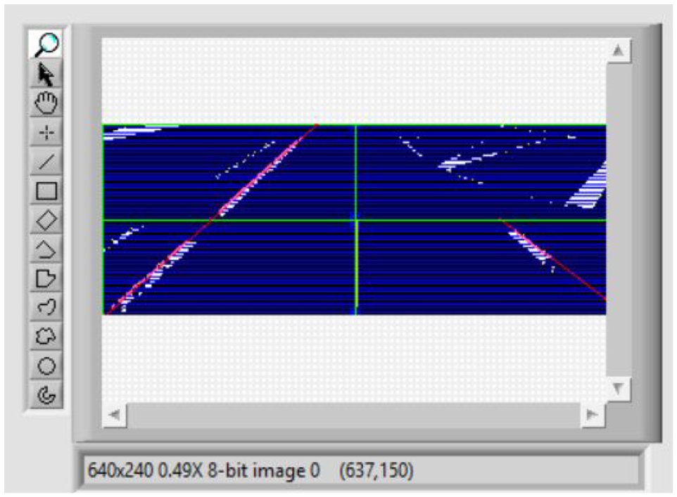
Lane detection result based on the proposed real time lane detection system.

Fully CNN lane detection simulation

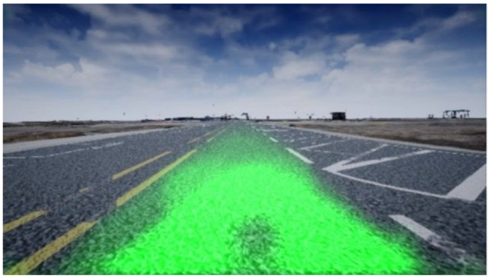
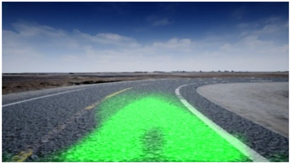
Based on description in Figure 7, the model is trained. After 10 epochs, the model is finished with MSE for training of 0.0024 and validation of 0.0024. After training, the result is saved in a json along with its weights. Two images are tested for lane detection, using deep learning based on CNN. The original images are sized as 640×480. Firstly, the images are resized to 80×160. Based on the training result, after prediction process, two images are shown in Figures 11 and 12, where the detected lane region is filled in green.

Figure 11.

Predicted result of lane detection based on fully CNN proposed in this paper.

Figure 12.

Predicted result of curved lane detection based on fully CNN proposed in this paper.

Based on the fully CNN method in,²¹ after training the model, test results are shown in Figures 13 and 14. After 20 epochs, the model finished with MSE for training of 0.0046 and validation of 0.0048. The results are worse than the results in Figures 11 and 12.

Figure 13.

Predicted result of straight lane detection based on CNN.

Figure 14.

Predicted result of curved lane detection based on CNN.

Trajectory planning and tracking simulation

In Figure 15, the reference points are defined as (0, 0), (0, –4), (20.5, 1), (30, 6.5), (40.5, 8), (50, 10) and (60, 6) in meters to generate the trajectory. Based on cubic spline interpolation method, the white trajectory is generated, where the white trajectory passes through the reference points. In the white trajectory, distances between two adjacent points are the same. Therefore, the vehicle can move in the constant speed. Obstacles are located at (20, 10), (30, 6), (30, 8), (35, 8), and (50, 3). When the vehicle tracks the white trajectory, the vehicle should avoid the obstacles. Using the optimization trajectory planning method based on frenet coordinate frame, the best trajectory is planned as the red lane. The trajectory avoids obstacles and finally tracks the generated path. Using the fuzzy sliding mode method, the vehicle’s yaw angle error is minimized as shown in Figure 16. In the frenet coordinate frame, initially, the vehicle is located at (1,0). Firstly, the vehicle should track the white path from its initial point, so error occurs. At time step 26-42, the vehicle should avoid obstacle, instead of tracking the white trajectory. Therefore, the vehicle should change its orientation to avoid obstacle, error occurs. However, finally, the vehicle yaw angle is close to zero.

Figure 15.

Vehicle trajectory planning and tracking.

Figure 16.

Vehicle’s Yaw angle.

As shown in Figure 17, pure pursuit trajectory planning method is compared with frenet optimized trajectory planning method. Passing through points (0, 0), (8, –4), (12, 2), (16, 4), (20, 2), (24, 0) and (27, 3) in meter, path is generated as blue lane in Figure 17. Based on frenet optimized trajectory planning method, the trajectory is planned as red lane. It is almost the same as the generated blue lane. However, based on pure pursuit trajectory planning method, green lane is planned. There is difference between the planned green lane and the generated blue lane, in x range of (0, 3).

Figure 17.

Comparison result between frenet optimized trajectory planning method and pure pursuit trajectory planning method.

In order to show the effectiveness of the trajectory, the proposed trajectory planning and tracking method is tested using a simulator. The simulator is made to demonstrate the performance on an outdoor autonomous vehicle. As shown in Figure 18(a), the left window is the simulator window, and the right window is shown the path based on the algorithm processing in LabVIEW. Based on the proposed path planning algorithm and fuzzy sliding control method for vehicle steer, the speed and steer commands are calculated. Then the commands are sent to the simulator based on RS232 communication. The vehicle in the simulator will move based on the speed and steer commands. Initially, the vehicle is located at (10 m, 0, 0). The light blue obstacle is located at (28 m, 0). The length of the vehicle is around 1.1 m. The target speed is defined as 10 km/h. The green lane is described as the generated path, which guarantees that the vehicle avoids the obstacle well. The dark blue lane is shown as the vehicles actual path. In Figure 18(b), the vehicle arrives at (20 m, –1 m) to avoid the predefined obstacle. In Figure 18(c), the vehicle tracks back to its predefined straight line. In Figure 18(d), the vehicle moves forward to its predefined straight line. The test simulator video is shown in https://www.dropbox.com/s/5up9w26hra799xv/path%20tracking.mp4?dl=0.

Figure 18.

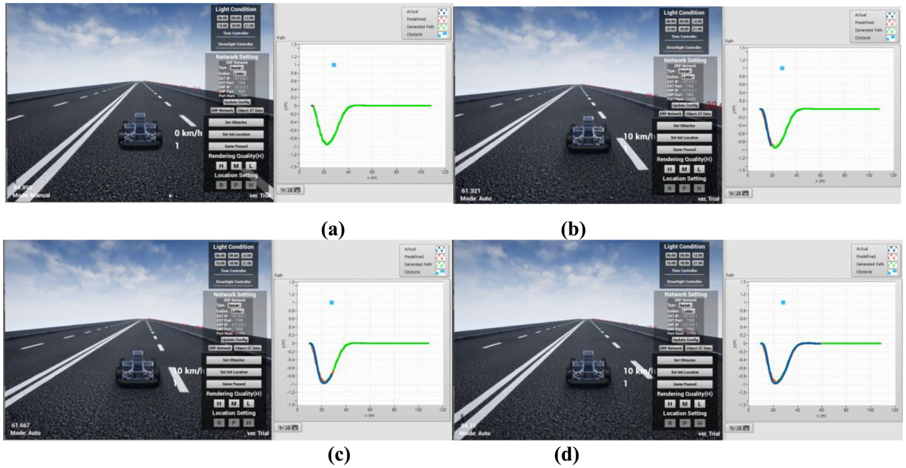
Test results of trajectory planning method and fuzzy sliding control method for vehicle steer using a simulator: (a) Initially, the vehicle is located at (10 m, 0, 0), (b) The vehicle arrives at (20 m, –1 m) to avoid the predefined obstacle, (c) The vehicle tracks back to its predefined straight line, and (d) The vehicle moves forward to its predefined straight line.

Experiment

The experiment is used to show the effectiveness of the trajectory planning method. As shown in Figure 19, the length of curved lanes is 4 m. The distance between two black lanes is 1.1 meter. Firstly, a curve path is generated, using cubic spline interpolation model. Then, the vehicle plans and tracks the trajectory successfully, based on optimization trajectory planning method in frenet coordinate frame. At t = 20 s, the vehicle passes through the curved part of the lane. At t = 30 s, the vehicle finishes the full path.

Figure 19.

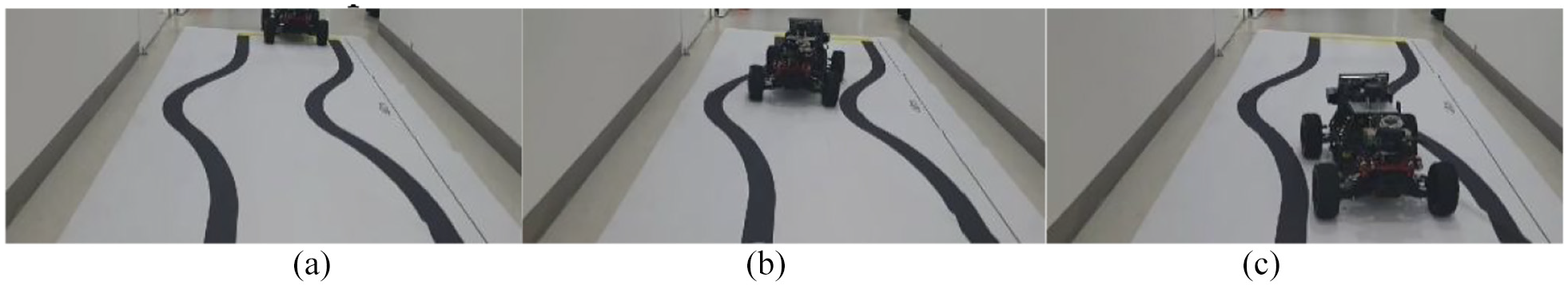
A vehicle plans and tracks the trajectory, based on optimize trajectory planning method in frenet coordinate frame. (a) t = 3 s, (b) t = 20 s and (c) t = 30 s.

Conclusions

In this paper, a real time lane detection system is proposed based on vision system functions, using webcam camera. In order to detect curve lanes, deep learning is applied for lane detection, based on fully CNN. The cubic spline interpolation method is used for path generation, based on GPS data, where distances between two adjacent path generation points are the same. Optimization trajectory planning method depending on frenet coordinate frame is used to plan a safe, easy and comfort trajectory. In addition, compared to the Cartesian coordinate frame, frenet coordinate frame simplifies the solution of road curve fitting problems, especially in the case of complex road environment. Fuzzy sliding control method for vehicle steering control is proposed. Finally, the simulation and experiment results show the effective performance of the proposed methods.

Footnotes

Handling Editor: James Baldwin

Declaration of conflicting interests

The author(s) declared no potential conflicts of interest with respect to the research, authorship, and/or publication of this article.

Funding

The author(s) received no financial support for the research, authorship, and/or publication of this article.

ORCID iD

Yanyan Dai

References

Pendleton

Andersen

, et al. Perception, planning, control, and coordination for autonomous vehicle. Machines 2017; 5: 1–54.

Thrun

Montemerlo

Dahlkamp

, et al. Stanely: the robot that won the DARPA Grand Challenge. J Field Robot 2006; 23: 661–692.

Chu

Lee

Sunwoo

. Local path planning for off-road autonomous driving with avoidance of static obstacles. IEEE Trans Intell Transp Syst 2012; 13: 1599–1616.

Waymo. Google self-driving car project, https://www.google.com/selfdrivingcar/

Tesla. Tesla motors: Model S press kit, https://www.tesla.com/presskit/

Newton

. Uber will eventually replace all its drivers with self-driving cars. Verge 2014; 5: 2014.

Peleshko

Ivanov

Sharov

, et al. Design and implementation of visitors queue density analysis and registration method for retail videosurveillance purposes. In: Proceedings of the IEEE first international conference on data stream mining & processing, Lviv, 23–27 August 2016, pp. 159–162. IEEE.

Nguyen

Kim

Jun

, et al. A study on real-time detection method of lane and vehicle for lane change assistant system using vision system on highway. Int J Eng Sci Technol 2018; 21: 822–833.

Gao

Duan

, et al. A practical method of road detection for intelligent vehicle. In: Proceedings of the 2009 IEEE international conference on automation and logistics, Shenyang, 5–7 August 2009, pp. 980–985. IEEE.

10.

Borkar

Hayes

Smith

. A novel lane detection system with efficient ground truth generation. IEEE Trans Intell Transp Syst 2012; 13: 365–374.

11.

Gong

Wang

, et al. A lane marking detection and tracking algorithm based on sub-regions. In: Proceedings of the 2014 international conference on informative and cybernetics for computational social systems, Qingdao, 9–10 October 2014, pp. 68–73. IEEE.

12.

Son

Yoo

Kim

, et al. Real-time illumination invariant lane detection for lane departure warning system. Expert Syst Appl 2015; 24: 1816–1824.

13.

National Instruments. IMAQ vision concepts manual. National Instruments, October 2000.

14.

Towards Data Science. Applied deep learning – Part 4: convolutional neural networks, https://towardsdatascience.com/applied-deep-learning-part-4-convolutional-neural-networks-584bc134c1e2

15.

Ozguner

Redmill

Acarman

. Autonomous ground vehicles. Norwood: Artech House, 2011.

16.

Dai

Choi

Lee

. Adaptive formation control and collision avoidance using a priority strategy for nonholonomic mobile robots. Int J Adv Robotic Syst 2013; 10: 1–14.

17.

French

. Advanced path planning for an autonomous SAE electric race car. Project report, 2014. Western Australia University.

18.

Werling

Ziegler

Kammel

, et al. Optimal trajectory generation for dynamic street scenarios in a Frenet Frame. In: Proceedings of the IEEE international conference on robotics and automation, Anchorage, AK, 3–7 May 2010, pp. 987–993. IEEE.

19.

Ivan

Iryna

Roman

, et al. Designing and simulation a motion control system of mobile robot based on fuzzy logic. Int J Adv Res Comput Eng Technol 2014; 3: 3143–3147.

20.