Multi-load cases topological optimization by weighted sum method based on load case severity degree and ideality

Abstract

Mechanical structures always bear multiple loads under working conditions. Topology optimization in multi-load cases is always treated as a multi-objective optimization problem, which is solved by the weighted sum method. However, different weight factor allocation strategies have led to discrepant optimization results, and when ill loading case problems appear, some unreasonable results are obtained by those alternatives. Moreover, many multi-objective optimization problems have certain optimization objective, and an evaluation formula to measure Pareto solution in the multi-objective optimization problem area is lacking. Regarding these two problems, a new method for calculating the weight factor is proposed based on the definition of load case severity degree. Additionally, an amplified load increment is derived and suggested in the minimum compliance with a volume constraint problem. Ideality is formulized from Pareto front to the ideal solution to evaluate the different optimization results. Benchmark topology optimization examples are solved and discussed. The results show that the load case severity degree is less affected by the different weighted sum functions and can avoid ill loading case phenomena, and the ideality of optimization result obtained by the load case severity degree is the best.

Introduction

Over recent decades, topology optimization has been indispensable in the lightweight design of engineering structures. Regarding these growing topology optimization methods,^1–4 the density method has been applied in software, such as ANSYS and Atair Optistruct. The pseudo density is defined as a design variable, and its value range is 0–1. Bendsøe ⁵ proposed the isotropic material with penalization (SIMP) model based on the density method. This model assumes a functional relationship between the elastic modulus and pseudo density, and a penalty factor is introduced to penalize the design variables to render the element density close to 0 or 1 simultaneously. The optimization algorithm or mathematical programming method is used to solve this model, where the elements with a pseudo density of 0 are removed and the elements with a pseudo density of 1 are retained, so the topological configuration is obtained. ⁶ Other methods are not sufficiently mature with respect to commercial applications.

In real engineering environments, mechanical structures usually bear multiple loads. Searching for the best mechanical property under each working condition is a multi-objective programming problem, ⁷ and it is a search process that finds the Pareto solutions. This article explores the single-parameter optimization problem under multiple working conditions. ⁸ The density topology optimization model is expressed as

$$\begin{array}{c}\min H(f_1(\rho ),f_2(\rho ),\cdots ,f_n(\rho ))\hfill \\ \mathrm{To}{g}_i(\rho )\ge g_0(\rho )\hfill \end{array}$$

(1)

where $\rho$ is the pseudo density of the finite element, $H(f(\rho ))$ represents the formulized objective function, $f_i(\rho )$ is the ith sub-objective function, n is the number of load cases, $g_i(\rho )$ is the constraint function, and $g_0(\rho )$ is the design threshold of the constraint function.

For the multi-objective programming problem, it is difficult to solve for every solution in the effective solution set. Therefore, the multi-objective optimization problem (MOP) is indirectly transformed into one or more single-objective optimization problems, and then one or better solutions can be obtained by easily solving the single-objective optimization problem. For multi-load cases topological optimization, the main solution strategies include the weighted sum method, the hierarchical sequence method, and the evolution algorithm.

In the hierarchical sequence method,^9,10 sub-objective problems are ranked as importance degrees. Therefore, the sorting results directly determine the final solution quality, and the importance sequence is more dependent on the designer’s subjective understanding. Booming evolution algorithms have been adopted in multi-load cases and multi-objective topological optimization.^11–15 Large search ranges and loose convergence criteria have been helpful for obtaining ideal Pareto solutions, but they are less efficient for multi-load cases topological optimization problems. The weighted sum method transforms the MOP into a single-objective optimization problem by constructing a new function equation that contains all the single-objective parameters. The monotonicity of the weighted sum function can guarantee noninferiority. Although the weighted sum method cannot obtain all the noninferior solutions, ¹⁶ one effective solution is enough for solving actual application problems. Moreover, this method is efficient and easy to implement. ¹⁷ Therefore, the weighted sum method is selected to solve the multi-load cases topology optimization problem in this research.

For multi-load cases topological optimization problems, in general, the weighted sum method includes the linear weighting method, weight-square method, compromise programming method, and weight-norm method, ¹⁸ as shown in equations (2)–(5), respectively

$$\begin{array}{c}\mathrm{linear}\mathrm{weighting}\mathrm{method}:\hfill \\ \mathrm{H}\left(\mathrm{f}\left(\mathrm{x}\right)\right)=\sum _{\mathrm{j}=1}^{\mathrm{p}}{\mathrm{w}}_{\mathrm{j}}\left({\mathrm{f}}_{\mathrm{j}}\left(\mathrm{x}\right)\right)\hfill \end{array}$$

(2)

$$\begin{array}{c}\mathrm{weight}-\mathrm{s}\mathrm{quare}\mathrm{method}:\hfill \\ \mathrm{H}\left(\mathrm{f}\left(\mathrm{x}\right)\right)=\sum _{\mathrm{j}=1}^{\mathrm{p}}{\mathrm{w}}_{\mathrm{j}}{({\mathrm{f}}_{\mathrm{j}}\left(\mathrm{x}\right)-{\mathrm{f}}_{\mathrm{j}}^0)}^2\hfill \end{array}$$

(3)

$$\begin{array}{c}\mathrm{weight}-\mathrm{norm}\mathrm{method}:\hfill \\ \mathrm{H}\left(\mathrm{f}\left(\mathrm{x}\right)\right)={\left(\sum _{\mathrm{j}=1}^{\mathrm{p}}{\mathrm{w}}_{\mathrm{j}}{({\mathrm{f}}_{\mathrm{j}}\left(\mathrm{x}\right)-{\mathrm{f}}_{\mathrm{j}}^0)}^{\mathrm{q}}\right)}^{1/\mathrm{q}}\hfill \end{array}$$

(4)

$$\begin{array}{c}\mathrm{compromise}\mathrm{programming}\mathrm{method}:\hfill \\ \mathrm{H}\left(\mathrm{f}\left(\mathrm{x}\right)\right)={\left\{{\sum _{\mathrm{j}=1}^{\mathrm{m}}{\mathrm{w}}_{\mathrm{k}}^{\mathrm{q}}\left[\frac{{\mathrm{C}}_{\mathrm{j}}\left(\mathrm{x}\right)-{\mathrm{C}}_{\mathrm{j}}^{min}}{{\mathrm{C}}_{\mathrm{j}}^{max}-{\mathrm{C}}_{\mathrm{j}}^{min}}\right]}^{\mathrm{q}}\right\}}^{\frac{1}{\mathrm{q}}}\hfill \end{array}$$

(5)

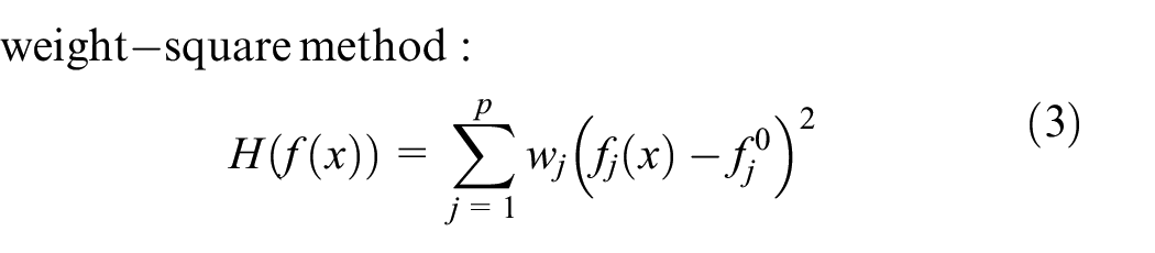
In terms of dimensions, the linear weighting method, weight-square method, and weight-norm method all maintain the dimensions of the original subgoal parameters, and the compromise programming method normalizes the subgoals to ensure uniform dimensions for each subgoal.

However, no matter which method is adopted, the problem of assigning weight factors is encountered. In structural optimization, the choice of weighting factors is crucial for obtaining a reasonable Pareto solution.^19–21 To obtain reasonable weight factors for multi-load cases optimization, the empirical method, average distribution, analytic hierarchy process (AHP), α method, and tolerance method have been used. The basic meaning of the weight factor was studied from the objective function by Marler and Arora, ¹⁷ wherein guidance rules for the weight factor setting of the linear weighting method were given. Based on gray system theory, Chen et al. ²² proposed a weight coefficient group evaluation method to obtain the optimal weight factor. Lan et al. ²³ distributed the weight factor based on the AHP, and this method was advantageous compared with the empirical method and orthogonal test method for optimizing a car body. Zhang et al. ²⁴ used the average distribution to assign a weight factor, which was used to solve the multi-load cases topological optimization of vehicle powertrain suspension brackets. Zou et al. ²⁵ drew a working condition risk radar map by calculating working condition indicators. The area of the radar chart was used to calculate the working condition risk index and then the weight factor was distributed. This method was effective because it optimized the forklift frame; however, the lack of threshold and ill loading cases were not considered. Ryu et al. ²⁶ proposed an adaptive weight determination method based on the concept of a hyperplane, so that the optimum design is found in the objective space. Sun et al. ²⁷ chose different weight factors to solve multi-load cases topological optimization problem of multi-cell tube, and these weight factors are determined by the statistical data of impact in actual environment.

Unfortunately, most researchers have paid more attention to the influence of different weight factors on the topological configuration and less attention to the influence of different weighted sum methods on the topology optimization objective results. Moreover, many optimization problems have certain optimization objective, such as minimum compliance or mass, but different optimization objective results are obtained by different weight factors and weighted sum methods; no criteria were given to choose one from these different optimization results.

When an engineering structure bears multiple loads, the load amplitude can be large or small. Once a small load can be omitted considering the transmission path or support position, the ill-load phenomenon is inevitable. For the ill loading case, Sui et al. ⁹ defined the loss of the load path caused by a large gap between the load values as the “ill loading case”; they solved the large load condition and small load condition using the idea of a weighted hierarchy based on the independent continuous mapping method (a topology optimization method proposed by Sui), and the weight factor was calculated by the load values. Sui et al. ²⁸ proposed an improved method to eliminate ill loading cases; a small load was amplified to enlarge the small load effect, but this method lacks a theoretical derivation and is not suitable for the density method. Qin and Yang ²⁹ studied the influence of the weight factor on the ill loading cases and topological optimization results. They proposed a gray theory method to accurately calculate the weight factor, but this method immoderately emphasized small load conditions, which led to an unreasonable optimization result. Therefore, a reasonable load amplification formula is necessary.

In this article, a multi-load cases optimization method based on the load risk degree and variable density theory is proposed. The main contents are organized as follows. In section “Weight factor calculation method,” the principles of the weight factor calculation methods are discussed in detail. In section “Weight factor calculation on the LCSD,” the weight factor calculation model based on the load case severity degree (LCSD) is proposed, a reasonable load increment is discussed, and a suggestion is given for ill loading case. In section “Ideality,” an evaluation equation of the topological optimization results based on ideality is proposed. In section “Numerical example,” all-sided numerical examples are presented, and the optimization results are discussed.

Weight factor calculation method

To comprehensively compare the advantages and disadvantages of different weight factor calculation methods, the principles of AHP, α method, and tolerance method are introduced briefly below.

AHP

When AHP method is used, designers first need to analyze the properties of every working condition. Subsequently, importance degrees of each working condition are sorted, and importance ratio of each subgoal is calculated through the scales shown in Table 1. Finally, judgment matrix W expressed as equations (6) is built ²³

$$\mathbf{W}=\left(\begin{array}{ccc}{\omega }_{11}\hfill & \dots \hfill & {\omega }_{1n}\hfill \\ \multicolumn{1}{c}{⋮}& \ddots \hfill & ⋮\hfill \\ \multicolumn{1}{c}{{\omega }_{n1}}& \cdots \hfill & {\omega }_{\mathrm{nn}}\hfill \end{array}\right)$$

(6)

wherein ${\omega }_i$ and ${\omega }_j$ (i, j = 1, 2) represent the importance factor of working conditions i and j, respectively, and ${\omega }_{\mathrm{ij}}={\omega }_i/{\omega }_j$ , which represents the relative importance of ${\omega }_i$ to ${\omega }_j$ .

Table 1.

The implication of importance scale.

Importance scale	Implication
1	Two elements are equally important
3	Compared with the two elements, the former is more important than the latter
5	Compared with the two elements, the former is more important than the latter obviously
7	Compared with the two elements, the former is more important than the latter strongly
9	Compared with the two elements, the former is more important than the latter extremely
2, 4, 6, 8	Intermediate value of above judgment
Reciprocal	If x is the ratio of the importance of i relative to j, 1/x represents the importance of j relative to i

Judgment matrix W is multiplied on the right by a vector consisting of all subgoal weight values $\mathbf{\omega }=({\omega }_1,{\omega }_2,\dots ,{\omega }_n{)}^T$ , as shown in equation (7). The weight factor can be calculated by solving this equation after normalization

$$\mathbf{W}\omega =\lambda \mathbf{\omega }2\Rightarrow (\mathbf{W}-\lambda I)\mathbf{\omega }=0$$

(7)

where $\lambda$ represents the eigenvalue of the judgment matrix.

Therefore, the weight factors are calculated by equations (6) and (7). However, the selection of the importance scale of each working condition is still subjective.

α method

The optimal solution of the single-objective optimization problem must be obtained first when the α method is used, as shown in equation (8)

$$\{\begin{array}{c}min{f}_i\left(x\right)\hfill \\ \multicolumn{1}{c}{s.t.x\in S}\end{array}i=1,2,3,\dots ,n$$

(8)

where x is the design variable and $f_i(x)$ represents the objective function result of the ith working condition. The best solution is defined as $x^{(k)}$ , and $f_i^{(k)}$ is defined as

$$f_i^{\left(k\right)}=f_i(x^{\left(k\right)})i,k=1,2,\dots ,n$$

(9)

The equations are defined as

$$\{\begin{array}{c}{\lambda }_1{f}_1^{\left(1\right)}+{\lambda }_2{f}_2^{\left(1\right)}+\cdots {\lambda }_n{f}_n^{\left(1\right)}=\alpha \hfill \\ \multicolumn{1}{c}{{\lambda }_1{f}_1^{\left(2\right)}+{\lambda }_2{f}_2^{\left(2\right)}+\cdots {\lambda }_n{f}_n^{\left(n\right)}=\alpha }\\ \multicolumn{1}{c}{\cdots \cdots }\\ \multicolumn{1}{c}{{\lambda }_1{f}_1^{\left(n\right)}+{\lambda }_2{f}_2^{\left(n\right)}+\cdots {\lambda }_n{f}_n^{\left(n\right)}=\alpha }\\ \multicolumn{1}{c}{{\lambda }_1+{\lambda }_2+\cdots {\lambda }_n=1,{\lambda }_i\succ 0}\end{array}$$

(10)

where ${\lambda }_1,{\lambda }_2,\dots ,{\lambda }_n$ are the weight factors of every working condition.

The weight factor calculated by the α method is reasonable when the gaps between subgoals are small; however, when there is a great gap between each working condition, the weight factors of some dangerous working conditions are almost zero. This result may lead to ill loading cases and unreasonable topological configurations.

Tolerance method

For the tolerance method, the variation ranges of each objective function are necessary, which is expressed as

$${\alpha }_i\le f_i\left(x\right)\le {\beta }_{i}i=1,2,\dots ,n$$

(11)

where ${\alpha }_i$ and ${\beta }_i$ represent the upper limit and lower limit of the objective function $f_i(x)$ , respectively. Therefore, the tolerance value $\mathrm{\Delta }{f}_i(x)$ and weight factors ${\omega }_i$ of each working condition are as follows

$$\mathrm{\Delta }{f}_i\left(x\right)=({\beta }_i-{\alpha }_i)/2i=1,2,\dots ,n$$

(12)

$${\omega }_i={1/\left[\mathrm{\Delta }{f}_i\left(x\right)\right]}^{2}i=1,2,\dots ,n$$

(13)

The tolerance method is suitable for calculating the weight factor when the upper limit and lower limit are certain, and it is easy to obtain these parameters during topological optimization.

Weight factor calculation on LCSD

LCSD

Engineering structures usually bear multiple loads. For instance, a car frame has requirements for side impact condition, frontal impact condition, and accelerating mode. A single-property optimization problem is discussed under multiple working conditions. When there are n load cases, objective functions are formulized by the weighted sum method. If all objective parameters are transferred to the minimization problem, then the optimum result of the formulized objective function is bigger than every single-objective result. Therefore, when the optimization result and limit value of the material property requirement (such as yield limit and damage limit) are closer under certain working conditions, the structure failure possibility is highest among all the load cases. Therefore, the weight distribution should be proportionately greater than the others. In this situation, we call the load case dangerous.

Therefore, the concept of LCSD is introduced to determine the weight factor. The LCSD is defined as the threat degree of optimized property parameters of each working condition to successfully achieve the optimal design goal (e.g. property requirement limit). The optimization objective, when the property limit value is definite, LCSD $\mathrm{\Delta }{\alpha }_i$ is calculated as

$$\mathrm{\Delta }{\alpha }_i=\frac{1}{|f_{lim}-f_i|}$$

(14)

where $f_{lim}$ is the objective property limit value and $f_i$ is the single condition optimization result of the ith working condition.

When the property limit value is not given, the objective function value is only required to be the largest or smallest. If the topological optimization result of one load case is the largest, then the LCSD of other working conditions are defined when the objective function is as small as possible, as shown in equation (15). The LCSD of other working conditions are defined when the objective function is as large as possible as equation (16)

$$\mathrm{\Delta }{\alpha }_i=\frac{f_i}{f_{max}}$$

(15)

$$\mathrm{\Delta }{\alpha }_i=\frac{f_{max}}{f_i}$$

(16)

Finally, the weight factor is calculated as equation (17)

$$\{\begin{array}{c}\mathrm{\Delta }{\alpha }_1:\cdots :\mathrm{\Delta }{\alpha }_n={\omega }_1:\cdots :{\omega }_n\hfill \\ \multicolumn{1}{c}{\sum _{i=1}^n{\omega }_i=1}\end{array}$$

(17)

where ${\omega }_i$ is the weight factor of the ith working condition.

Obviously, if the sub-objective function value of one case is much larger/smaller than others, then the topological optimization results of some working conditions will have large gaps compared with the property limit values. The LCSD of this working condition, calculated by equations (16) and (17), is close to 0, which means that those working conditions are extremely safe, and the weight factors are also close to 0. This result may lead to the disappearance of the load path of some load cases and an unreasonable topological result, ⁹ especially when there are supporting spots along the path. Therefore, the case where the load ratio is 100–1000 is discussed in this article.

A straightforward way to deal with the ill loading cases is to amplify a small load. The property variation is different when the load values of a small load and a large load change $\mathrm{\Delta }F$ simultaneously. Compared with the large load, the same change in the small load causes a dramatic change in the structure property. Therefore, the load increment $\mathrm{\Delta }{P}_i$ is applied to each load to reduce the structural property disparity. $A_i$ is used to represent the amplification coefficient (AC) of the property parameter in the ith working condition. This amplification coefficient reflects the change times when the load increment is $\mathrm{\Delta }{P}_i$

$$A_i=\frac{f_i^{\mathrm{new}}-f_i}{f_i}$$

(18)

where $f_i^{\mathrm{new}}$ is the structural property after changing the load. Therefore, the modified weight factor calculation equation is renewed in equation (19)

$$\{\begin{array}{c}{A}_1\mathrm{\Delta }{\alpha }_1:\cdots :A_n\mathrm{\Delta }{\alpha }_n={\omega }_1:\cdots :{\omega }_n\hfill \\ \multicolumn{1}{c}{\sum _{i=1}^n{\omega }_i=1}\end{array}$$

(19)

Load increment selection

Although the load increment can overcome the ill loading case, an unreasonable selection of the load increment will lead to two results: (1) the load increment is too small so that the ill loading case is not overcome and (2) the load increment is too large to avoid the influence of the load path of the large load condition, which leads to an unsatisfactory optimization result. Therefore, the load increment must be reasonably selected to obtain a reasonable topological result.

In the engineering topology optimization field, the problem of the minimum compliance with a volume constraint (MCVC) is discussed mostly. Therefore, the load increment value is discussed under the MCVC.

The working condition with the smallest load value $P_{min}$ is selected as the first working condition; then, the order of working conditions is defined from the smallest to the largest. The load value of the jth working condition can be expressed as

$$P_j={\lambda }_j{P}_{min}$$

(20)

where $P_j$ is the load value of the jth load case and ${\lambda }_j$ is the load ratio of the jth case to the smallest load value, ${\lambda }_j\ge 1$ . When the smallest load value $P_{min}$ changes with $x{P}_{min}$

$$P_{min}^Z=P_{min}+x{P}_{min}=(x+1)P_{min}x\in R$$

(21)

where $P_{min}^Z$ is the smallest load value after change and x is the load increment coefficient. Other loads can be developed as

$$P_j^Z={\lambda }_j{P}_{min}+x{P}_{min}\Rightarrow P_j^Z={\lambda }_j(1+\frac{x}{{\lambda }_j})P_{min}$$

(22)

where $P_j^Z$ is the load value of the jth working condition after the change.

According to finite element theory, the compliance and load can be simplified as

$$\{\begin{array}{c}{C}_j=\frac{1}{2}{{\mathbf{U}}_j}^T\mathbf{K}{\mathbf{U}}_j\hfill \\ {\mathbf{P}}_j=\mathbf{K}{\mathbf{U}}_j\hfill \end{array}$$

(23)

where $C_j$ is the initial compliance of the ith working condition, ${\mathbf{U}}_j$ is the displacement vector of the ith working condition, and K is the stiffness matrix. The relationship between the compliance and load can be described as

$$C_j=\frac{1}{2}{{\mathbf{P}}_j}^T{\mathbf{K}}^{-T}{\mathbf{P}}_j$$

(24)

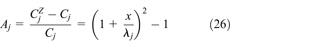
In equation (23), if the load value of the ith working condition is increased by $1+(x/{\lambda }_j)$ times, then the compliance can be developed as

$$C_j^Z={(1+\frac{x}{{\lambda }_j})}^2{C}_j$$

(25)

where $C_j^Z$ is the compliance of the jth working condition after changing the load. Then, the amplification factor is calculated as

$$A_j=\frac{C_j^Z-C_j}{C_j}={(1+\frac{x}{{\lambda }_j})}^2-1$$

(26)

Because of the lack of the limit value, equations (16), (19), and (26) and the ratio of the weight factor is simultaneously calculated as

$$\frac{{\omega }_1}{{\omega }_j}=\frac{A_1\times \mathrm{\Delta }{\alpha }_1}{A_j\times \mathrm{\Delta }{\alpha }_1}=\frac{{(x+1)}^2-1}{{(1+\frac{x}{{\lambda }_j})}^2-1}\times \frac{C_1^o}{C_j^o}=h(x,{\lambda }_j)\times r_j$$

(27)

where $h(x,{\lambda }_j)$ is the relative amplification coefficient (RAC), which reflects the amplification degree of the first working condition compared to the jth working condition, and RAC shows the true amplification effect of the smallest load. $C_1^o$ and $C_j^o$ are the optimization results of the first and ith load cases, respectively, and $r_j$ , a constant, is the optimization objective result ratio of the jth working condition and the first working condition.

Obviously, the ratio of weight factors of the first working condition compared to the ith working condition is an expression about the RAC and is enlarged by an increasing amplification factor. When the load ratio ${\lambda }_j=1$ , the RAC is constantly 1. That is, when the external load values under all working conditions are equal, the ratio of the weighting factors of each working condition is equal to the ratio of the topological optimization results of the single working conditions, and the load increment is independent of the weighting factor.

When the load ratio ${\lambda }_j>1$ , the ratio of the weight factors of each working condition will change with changing load increment, that is, multiple weight factors will be obtained by equation (19). Figure 1 describes the relationship of the RAC, load increment factor, and load ratio. When the load increment factor is determined, the RAC increases with increasing load ratio, and the RAC is close to convergence when the load increment factor is greater. This finding means that the impact of the load ratio on the structure is almost eliminated, and the load path and property of the danger working condition will be greatly affected.

Figure 1.

Relationship of the RAC and load increment coefficient.

To minimize the influence of the load increment, a smaller load increment is required to obtain a larger RAC, so the derivative of the RAC to the load increment factor is necessarily calculated, as shown in equation (28). Figure 2 describes the function image of this derivative. From this figure, the growth rate of the RAC is most remarkable when the load increment factor is zero, and the value of the growth rate is $({\lambda }_j-1)/2$ . However, as the load increment increases, the RAC growth rate gradually decreases; that is, as the load increment increases, the amplification effect obtained by increasing the same load increment decreases

$$\frac{\partial h(x,{\lambda }_j)}{\partial x}=2{\lambda }_j^2\times \frac{{\lambda }_j-1}{{(x+2{\lambda }_j)}^2}$$

(28)

Figure 2.

Growth rate of the RAC.

When the growth rate of the RAC is less than β times the maximum value, the load increment is defined as a weak load increment (Figure 2). Conversely, the load increment is defined as a strong load increment, and according to this definition, the load increment factor is calculated as

$$x_j=(\frac{1}{\sqrt{\beta }}-1)\times 2{\lambda }_j\beta \in (0,1)$$

(29)

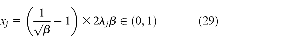
Numerical calculation experiments show that $\beta =0.95$ is ideal and $x_j=0.052{\lambda }_j$ . Therefore, the load increment under the MCVC is recommended as

$$\mathrm{\Delta }{P}_j=0.052{\lambda }_j{P}_{min}=0.052P_j$$

(30)

Multi-load cases topological optimization based on the LCSD

The overall process of the optimization method based on the LCSD is illustrated in Figure 3.

• Step 1. A single working condition is carried out, and objective function values before and after optimization $f_i$ and $f_i^s$ are obtained.

• Step 2. The severity degrees of each working condition are calculated with equation (15) or (16).

• Step 3. Judge whether there is an ill loading case according to the optimization result, if not, go directly to step 6; otherwise, go to step 4.

• Step 4. Select the minimum load under all working conditions. It is used to calculate the load increment $\mathrm{\Delta }{P}_i$ through equation (30).

• Step 5. The structure property $f_i^{\mathrm{new}}$ is analyzed after applying the load increment, and the amplification coefficient $A_i$ is calculated with equation (18).

• Step 6. The amended weight factor is calculated by equation (17) or (19).

• Step 7. The multi-load cases topological optimization model is structured and solved.

Figure 3.

Flow chart of the multiload case topological optimization method.

Ideality

Different optimization results are obtained by different weight factors; those optimization results constitute different Pareto fronts, and designer will choose the appropriate solution. However, many optimization problems have their fixed optimization goals. For example, when compliance is the objective function, although the flexibility cannot be 0, the smaller the flexibility, the better (generally, it will bigger than the single working condition after optimization value of weight-compliance), so these MOPs have only one optimal solution. A simple comparison of the weighted objective value cannot reflect the merits of the optimization result because of the coupling between the weight factor and every objective function value. Therefore, ideality is introduced to evaluate the different optimization results. Ideality is defined as the difference degree between the optimization result and ideal solution, which reflects the proximity of the Pareto front to the ideal solution. The smaller the distance between Pareto and the ideal solution, the larger the ideality, as illustrated in Figure 4.

Figure 4.

Ideality.

Since the weight factor has already expressed the designer’s preference, the weight factor is not considered when establishing the ideality computing model. Ideality I is defined as

$$I=\frac{1}{{\left(\sum _{j=1}^n{(f_j^m-f_j^s)}^2\right)}^{1/2}}$$

(31)

where $f_j^m$ is the multi-load cases topological optimization result of the jth working condition and $f_j^s$ is the ideal solution of the jth working condition.

When there is a property requirement limit, it is taken as an ideal solution. However, in general, requirement limits do not exist. Because the optimal calculation of conflict factors leads to a compromise answer, the optimization result of multi-load cases optimization is worse than the single result, as illustrated as

$$\{\begin{array}{c}{f}_j^s\prec f_j^m\mathrm{objective}\mathrm{function}\mathrm{is}\mathrm{as}\mathrm{small}\mathrm{as}\mathrm{possible}\hfill \\ \multicolumn{1}{c}{f_j^s\succ f_j^m\mathrm{objective}\mathrm{function}\mathrm{is}\mathrm{as}\mathrm{large}\mathrm{as}\mathrm{possible}}\end{array}$$

(32)

where $f_j^s$ and $f_j^m$ represent the optimization result of the jth working condition after single case topological optimization and multi-load cases topological optimization, respectively. Therefore, the ideal solution is obtained as

$$\mathbf{T}=(f_1^s,f_2^s,f_3^s...f_n^s)$$

(33)

where T is the set of ideal solutions.

In particular, when the property requirement limit does not exist, if the optimized result of a working condition is worse than the others, then it is taken as the ideal solution, as shown in equation (34)

$$\{\begin{array}{c}\mathbf{T}=(f_i^s\cdots f_i^s)\hfill \\ \multicolumn{1}{c}{s.t.f_i^s>f_j}\end{array}i,j=1,2,\dots ,n;i\ne j$$

(34)

where $f_i^s$ is the optimized structural property and $f_j$ is the initial structural property.

Numerical example

Ill loading case problem of the LCSD

Example 1: As illustrated in Figure 5, the plate size is 200 mm × 100 mm, the elasticity modulus is 20 GPa, and Poisson’s ratio is 0.2. The plate is subjected to two working conditions: (1) the first load in the upward vertical direction $p_1=1\mathrm{N}$ and (2) the second load in the downward vertical direction $p_2=100\mathrm{N}$ . The volume fraction of the constraint condition is 0.4, and the minimum compliance is set as the objective function. Compromise programming is used to construct the objective weighted sum as equation (5).

Figure 5.

Example 1 with P₂/P₁ = 100.

Topological optimization is carried out under two working conditions, and the severity degree is calculated by equation (15). Table 2 shows the optimization results and severity degrees of each load case. Obviously, the severity degree of P₂ is 10,000 times larger than that of P₁, and there are ill loading case problems. Therefore, the weight factors of the two load cases are calculated by equations (17) and (19). The topological configuration is enumerated in Table 3. As we can see, the topological configuration based on LCSD is reasonable.

Table 2.

Topological optimization result and severity degree.

	Load case 1	Load case 2
Minimum compliance	1.80E−05	1.80E−01
Maximum compliance	7.25E−05	7.25E−01
Severity degree	1.00E−04	1.00

Table 3.

Topological result based on LCSD.

Load increment (N)	Weight factor	Topological configuration
0	(10−4, 1–10−4)
5.2	(0.034, 0.966)

LCSD: load case severity degree.

Example 2: As illustrated in Figure 6, the size and material properties are the same as in Example 1. The plate is subjected to two working cases: (1) the first center load in the downward vertical direction is $p_1=1000\mathrm{N}$ and (2) the second load of the right corner in the down vertical direction is $p_2=1\mathrm{N}$ . The volume fraction is 0.4, the minimum compliance is set as the objective function, and compromise programming is used to construct the objective function.

Figure 6.

Example 2 with P₂/P₁ = 1000.

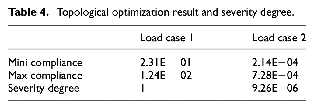
Topological optimization is carried out under two working conditions, and the severity degree is calculated by equation (15). Table 4 shows the optimization results and severity degrees of each working condition, and the optimization results are shown in Table 5. As we can see, when the weighting factors are calculated by LCSD, the topological result retains the lathy load path caused by $p_2$ , which perfectly proves the versatility of avoiding ill loading cases.

Table 4.

Topological optimization result and severity degree.

	Load case 1	Load case 2
Mini compliance	2.31E+01	2.14E−04
Max compliance	1.24E+02	7.28E−04
Severity degree	1	9.26E−06

Table 5.

Topological result based on LCSD.

Load increment	Weight factor	Topological configuration
0	(1–10−6, 10−6)
52	(0.8, 0.2)

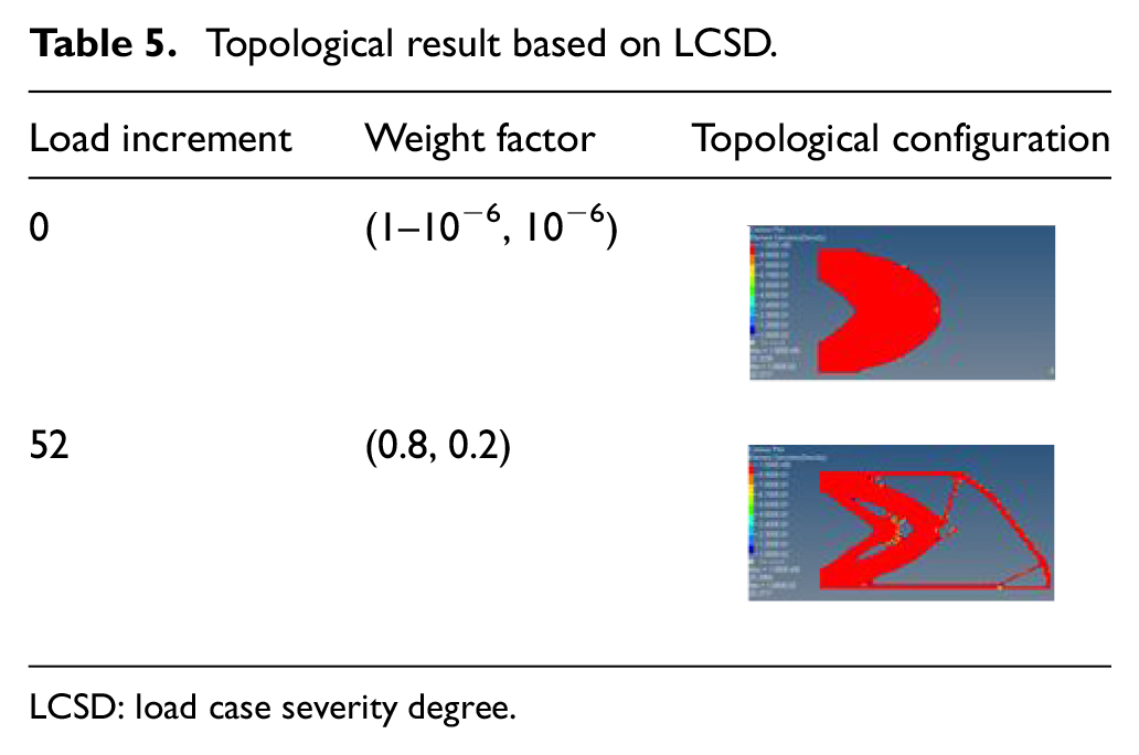
LCSD: load case severity degree.

Effect of different weighted sums on the LCSD

When the weight factor is determined, different weighted sums lead to diverse results. Therefore, it is necessary to compare the topological configurations and optimal effects under different weighted sums and different weight factor calculation methods.

Example 3: The structure property of each working condition is quite different. As shown in Figure 7, the size of the plate is 200 mm × 100 mm, the elasticity modulus is 20 GPa, Poisson’s ratio is 0.3, and the left side is fully fixed. The plate is subjected to two working cases: (1) the center of the plate is applied to a vertical load $p_1=1\mathrm{N}$ and (2) the middle of the right side is applied to a vertical load $p_2=100\mathrm{N}$ .

Figure 7.

Example 3 with P₂/P₁ = 100.

Example 4: As shown in Figure 8, the unit cantilever plate’s size is $\sqrt{2}\times (\sqrt{2}/2)$ mm, the elasticity modulus is 0.1 MPa, Poisson’s ratio is 0.3, and the left side is completely fixed. The plate is subject to two cases: (1) the middle of the right side is subjected to a downward vertical load $p_1=1\mathrm{N}$ and (2) the bottom right corner is subjected to a load $p_2=1\mathrm{N}$ in the downward vertical direction.

Figure 8.

Example 4 with P₂/P₁ = 1.

Since there is no threshold value for the stiffness, the topology optimization of the cantilever plate is carried out in a single case. First, the volume ratio constraint is set as 0.4, and the minimum compliance is set as the objective function. The severity degree of each working condition is calculated, and the ideal solution is derived by equation (31). Table 6 shows the optimization results and severity degree of each load case. The severity degree of case 2 in Example 3 is 10,000 times larger than the value of case 1, which means that there is an ill loading case phenomenon. The load increment is calculated by equations (18), (19), (30), and (32), and the AC, the weight factor, and the ideal solution are shown in Table 7.

Table 6.

Compliance result and severity degree of a single working condition.

	Example 3		Example 4
	Load case 1	Load case 2	Load case 1	Load case 2
Minimum compliance	2.310E−5	1.931	38.632	42.771
Maximum compliance	1.240E−4	2.249	124.972	145.558
Severity degree	1.2E−5	1	0.903	1

Table 7.

Result of the load increment, amplification coefficient, weight factor, and ideal solution.

	Example 3		Example 4
	Load case 1	Load case 2	Load case 1	Load case 2
Load increment (N)	5.2		0
Amplification coefficient	37.440	0.107	0	0
Weight factor	0.004	0.996	0.48	0.52
Ideality	(1.931, 1.931)		(28.570, 31.471)

The linear weighting method, weight-square method, weight-norm method, and compromise programming method are used to construct the weighted sum method by equations (2)–(5), respectively. Additionally, the weighting factors are calculated by the LCSD, AHP, tolerance method, empirical method, and α method, at the same time, and according to empirical method, w₁ = 0.2, 0.4, 0.6, and 0.8. Different topological configurations were obtained, as shown in Tables 8 and 9. When the ratio of the severity degree is close to 1E+5, the weight factors obtained using the α method are W₁ = 0.99997 and W₂ = 0.00003; that is, the weight factor of the small load condition is too large, so when there is an ill loading case problem, the α method is not suitable to calculate the weight factor.

Table 8.

Multi-load cases topological optimization result in Example 3.

	Compromise programming method	Linear weighting method	Weight-square method	Weight-norm method
LCSD W1 = 0.004 W2 = 0.996	f min = 0.0151	f min = 1.9243	f min = 3.1153e−6	f min = 5.7348e−4
AHP W1 = 0.17 W2 = 0.83	f min = 0.0386	f min = 1.6041	f min = 3.9229e−6	f min = 6.3229e−4
W 1 = 0.2 W2 = 0.8	f min = 0.0415	f min = 1.5462	f min = 3.7248e−6	f min = 6.3505e−4
Tolerance method W1 = 0.21 W2 = 0.79	f min = 0.0628	f min = 1.5269	f min = 3.6673e−6	f min = 6.2588e−4
W 1 = 0.4 W2 = 0.6	f min = 0.0719	f min = 1.1598	f min = 2.3519e−6	f min = 4.9837e−4
Average method W1 = 0.5 W2 = 0.5	f min = 0.0779	f min = 0.9665	f min = 1.8881e−6	f min = 4.3601e−4
W 1 = 0.6 W2 = 0.4	f min = 0.0725	f min = 0.7733	f min = 1.3815e−6	f min = 3.7617e−4
W 1 = 0.8 W2 = 0.2	f min = 0.0738	f min = 0.3867	f min = 6.9709e−7	f min = 2.9928e−4

LCSD: load case severity degree; AHP: analytic hierarchy process.

Table 9.

Multi-load cases topological optimization result in Example 4.

	Compromise programming method	Linear weighting method	Weight-square method	Weight-norm method
W 1 = 0.2 W2 = 0.8	f min = 0.0104	f min = 43.7317	f min = 1.988	f min = 1.4146
AHP W1 = 0.25 W2 = 0.75	f min = 0.0103	f min = 43.7021	f min = 2.2606	f min = 1.5041
W 1 = 0.4 W2 = 0.6	f min = 0.0123	f min = 43.3916	f min = 2.5151	f min = 1.6432
LCSD W1 = 0.48 W2 = 0.52	f min = 0.0132	f min = 43.0150	f min = 2.6373	f min = 1.6629
Average method W1 = 0.5 W2 = 0.5	f min = 0.0133	f min = 43.1584	f min = 2.7786	f min = 1.6973
α method W1 = 0.54 W2 = 0.46	f min = 0.0136	f min = 43.0116	f min = 2.8580	f min = 1.7487
Tolerance method W1 = 0.58 W2 = 0.42	f min = 0.0154	f min = 42.7451	f min = 2.7681	f min = 1.6979
W 1 = 0.6 W2 = 0.4	f min = 0.0153	f min = 42.5371	f min = 2.8435	f min = 1.7236
W 1 = 0.8 W2 = 0.2	f min = 0.0136	f min = 41.5741	f min = 3.3393	f min = 1.9122

AHP: analytic hierarchy process; LCSD: load case severity degree.

The topology optimization results of Example 3 and Example 4 are shown in Tables 8 and 9, respectively. According to those optimization results, the optimized configurations are divided into two and three regions for comparison, as shown in Figure 9.

Figure 9.

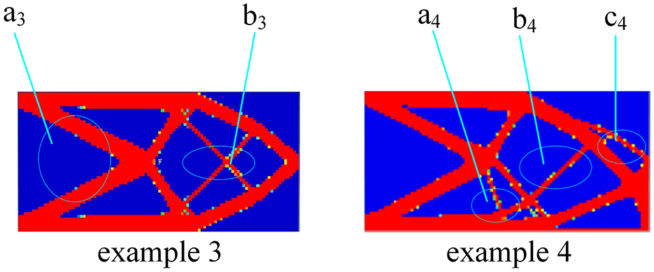
Area division of the optimization results.

The differences in the topology configurations in Tables 8 and 9 are summarized in Table 10. For the tolerance method and empirical method, the most different areas include a₃, b₃, a₄, b₄, and c₄. This result means that the topology optimization configuration is more affected by weighted sum selection when the two methods are used. For the AHP and average method, the most different areas are a₃, b₃, and a₄, which means that these methods are only suitable for the condition where there are no ill loading case problems. For the LCSD, the most different area is a₄, and there are the fewest different areas, which means that the topology optimization configuration is less affected by the weighted sum selection, especially when there is an ill loading case problem.

Table 10.

Different areas under different weighted sum methods.

	Different areas
	Example 3	Example 4
AHP	a3, b3	a4
Tolerance method	a3, b3	a4, b4, c4
α method	–	a4
Empirical method	a3, b3	a4, b4, c4
Average method	a3, b3	a4
LCSD	0	a4

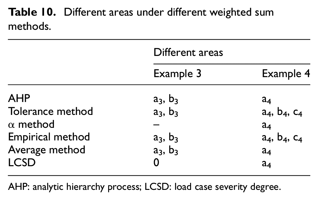
AHP: analytic hierarchy process; LCSD: load case severity degree.

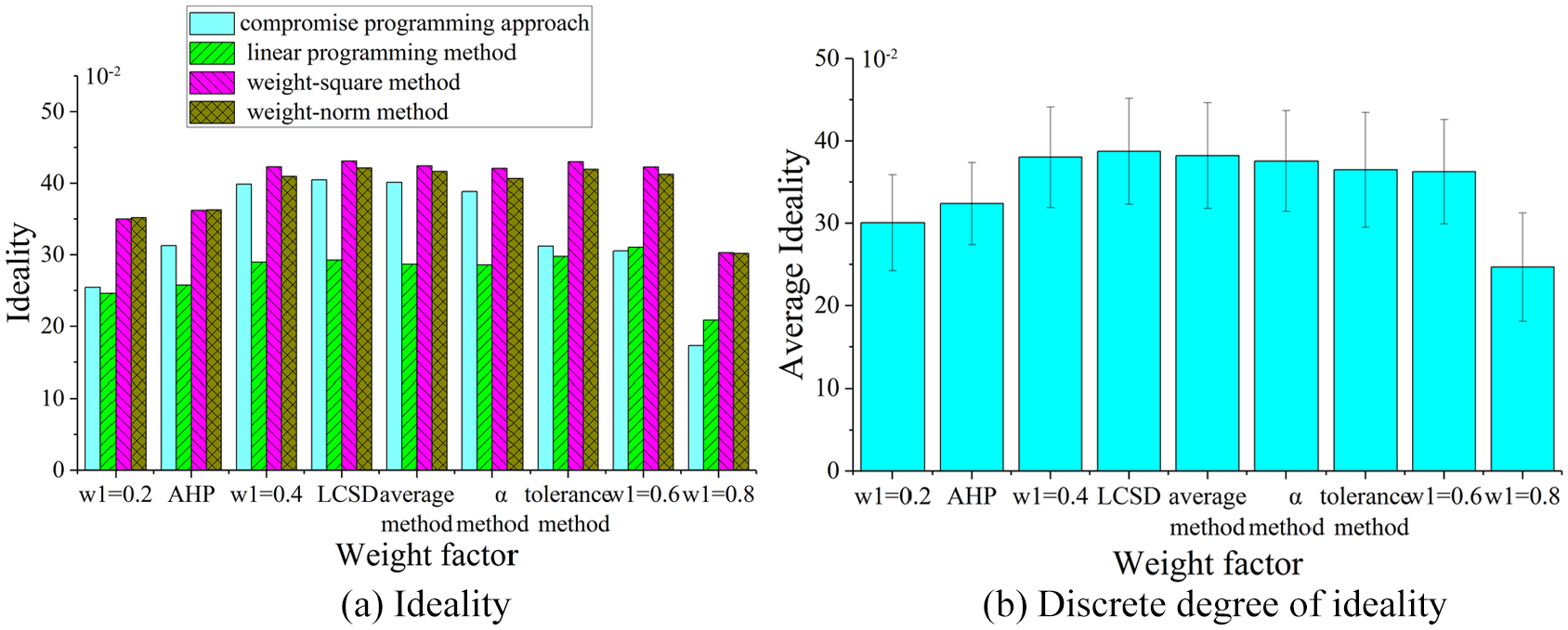
The ideal analysis results of Tables 8 and 9 are illustrated in Figures 10 and 11, respectively. The standard deviation is calculated for these idealities when the weight factor is determined, and the weighted sum is different because it reflects the discrete degree between individuals, as shown in Figures 10(b) and 11(b). The longer the error bar is, the larger the standard deviation is and the more discrete the results are.

Figure 10.

Optimization results analysis in example 3.

Figure 11.

Optimization results analysis in example 4.

As shown in Figure 10(b), the average ideality is different between the load cases. Obviously, if the empirical method is used, then the optimization result is greatly affected by the experience of the designer, which means that the designer decides how the optimization result is affected by the different weighted sums. If the weight factors are distributed by the average method, then the average ideality is smaller, the standard deviation is larger, and the optimization results are not ideal and are unstable. If using the AHP or tolerance method, then the average ideality is larger and the standard deviation is smaller; that is, the two methods are not affected by the weighted sum, and the optimization results obtained by the two methods are more ideal. When using the LCSD, although the standard deviation is larger, the average ideality is largest, and the smallest ideality is close to the average ideality of other methods, which means that the optimization result obtained by the LCSD is best.

The structural properties of each load case are not much different, as shown in Figure 11. According to Figure 11(a), when weight factors are certain, the ideals of the optimization results based on different weighted sums are different. Furthermore, the ideals based on the compromise programming method and linear weighting method are worse than the ideals based on the compromise programming method and linear weighting method weight-square method and weight-norm method, and the ideal based on the linear weighting method is the worst. According to Figure 11(b), the average ideal based on the LCSD is largest, although its standard deviation is larger, which means that the optimization result is the best according to the LCSD. The standard deviation based on the AHP is the smallest, but the average ideal of this method is also smaller. These results mean that the optimization results based on the AHP and different weighted sums are the most similar and are not the best results.

In summary, the empirical method is determined by the designer’s experience, which will lead to great uncertainty; the average method cannot obtain an ideal solution, especially if there is a great gap between different load cases. The AHP is affected by the weighted sum when the structural property of each load case is not much different; it still cannot avoid subjective factors. The α method cannot be used when ill loading cases appear. The tolerance method is almost unaffected by the evaluation, but the average ideality is not the best. Compared with the above methods, regardless of the working conditions of the structure, if the weight factor is determined by the LCSD, then the average ideality is largest and the standard deviation is smaller. That is, the optimization result is best and less affected by the weighted sum selection.

Conclusion

1. Based on the idea of the proximity degree with an objective threshold, the severity degree is proposed to measure the failure risk of load cases. A weighting factor determination method considering the severity degree of a load case is proposed. The initial and optimized objective function values are used to calculate the severity degree, and the ratio of severity degrees is equal to the ratio of weight factors.

2. To avoid ill loading case problems, load increments are used. The relationship between the RAC and load increment is derived, and the recommended formula of load increment is given. Numerical examples are used to discuss effectiveness of the method for dealing with the ill-conditioned problem.

3. Topological configuration is affected by different weighted sum methods because of the unreasonable weight factor. When the weight factor is calculated by the tolerance method and empirical method, the topological configuration is most affected by the weighted sum function; when the LCSD is used, the impact is minimal, especially when an ill loading case problem appears.

4. To measure multiple objective optimization results, a definition and calculation method of ideality are proposed based on the distance between the multi-objective optimization result and ideal solution, and sub-objective values based on different weighted sums are compared and discussed. The LCSD method proposed in this article is rarely affected by the weighted sum function and effectively avoids ill loading case problems. The average ideality of this method is the largest, and the discrete degree of the sub-objective value is smaller. Therefore, this method is more suitable to calculate the weight factor; additionally, this method can also be used to solve the dynamic response optimization problem and size optimization problem.