Simulations of unsteady flows with adsorption equilibrium in dynamic axial compression column

Abstract

Simulated moving bed chromatography process, which is a multicolumn chromatography process, has been used in various industrial applications. Dynamic axial compression columns are key elements in simulated moving beds, and their flow characteristics are worth exploring using state-of-the-art numerical methodologies. In this study, new fluid distributors for the dynamic axial compression column were designed and fabricated based on mass conservation in fluid mechanics and the computer-aided design in the preliminary stage. Computational fluid dynamics was employed to resolve the flow field, and the numerical chromatograms were validated by laboratory experiments. For the computational fluid dynamics–based simulation of flow in the dynamic axial compression, the transient laminar flow fields were described by the momentum and species transport equations with Darcy’s law to model the porous zone in the packed bed. In addition, reverse engineering processes were applied to obtain the unknown physical parameters, such as viscous resistance and adsorption equilibrium coefficients. Moreover, including the adsorption equilibrium equation in the fundamental governing equations made the simulated results agree with the experimental data in chromatograms, providing a more feasible result for practical applications.

Introduction

The simulated moving bed (SMB) technique is considered a multicolumn chromatography process. It has been applied in various industrial fields, such as foods, petrochemicals, fine chemicals, and pharmaceuticals. ¹ In the SMB process, periodically shifting the inlet and outlet nodes simulates the counter current movement of the adsorbent bed to the direction of the flow for certain time intervals. In addition, the dynamic axial compression (DAC) column is the key element in the SMB. In this column, different solutes can be separated from the solvent due to their different flow characteristics in packed beds. For most preparative and process-scale chromatographic columns, the DAC column ends include distributors (or collectors) and frits to distribute (or collect) fluid over the column cross-section. Figure 1 displays an illustration of the DAC column with a distributor, a collector, and two frits. Figure 1(a) is a sketch from computer-aided design (CAD), and the components are detailed in Figure 1(b). The SMB process can achieve low solvent consumption and high productivity. ² Therefore, it allows significantly higher yield and purity compared with a batch chromatography.^3,4

Figure 1.

Sketch of the single DAC column: (a) illustration of CAD and (b) detailed fluid distributor position.

The pre- and post-column geometries play a key role in the combined effects of the DAC column dynamics for chromatography. At the column inlet, a cross-sectional plug flow distribution should be achieved through careful design to allow acceptable separation efficiency.^5,6 Thus, the distributor at the column header is critical to provide even flow and consequently improve the column efficiency. Moreover, appropriate packing materials (porous medium) must be selected and the column must be carefully packed to retain a flow pattern as close as possible to even flow.^7,8 If these factors are not considered, band distortion and unsymmetrical peaks would be observed because a faulty header design can lead to flow misdistribution.^6,9 Furthermore, DAC columns tend to be of low length over diameter (L/D) for high-productivity considerations, which results in poor flow distribution and reduces the column efficiency. Manufacturers have been devoted to improving the distributor’s performance to increase the efficiency of their products from DAC columns.^10,11

Nowadays, numerical techniques, such as the homotopy analysis method ¹² and computational fluid dynamics (CFD), ¹³ are employed to solve fluid flow through a porous medium. In this article, CFD is adopted to simulate the flow field inside the DAC column. CFD has been known for over 30 years as a practical and reliable tool to solve heat and mass transfer problems in various industrial processes. ¹⁴ Moreover, CFD-based modeling and numerical simulation have been adopted to explore the transport phenomena in the preparative chromatography column.^13,15–17 In this study, CFD is proposed to explore the hydrodynamics of DAC columns based on up-to-date approaches of flow characterization and then to figure out numerical treatments that can be beneficial to simulations. In this research, CFD is used to access information on the inside of the DAC column, and the flow is considered to be laminar due to low flow speed with adsorption equilibrium in the micro-particle-packed column.^8,18 In the section of physical modeling, the DAC structure is introduced, the rules of innovative design for distributors are proposed, and experimental setup and procedures are described. The section of mathematical modeling comprises governing equations and their numerical treatments and the CAD and CFD techniques to simulate flow fields in the DAC column. The results and discussions are presented thereafter, which include patterns of new distributors and comparisons of experimental and numerical data. Improvements from considering adsorption equilibrium are also depicted in this section. The conclusions, including the contributions of the study and future works, are presented in the final section.

Physical modeling

The DAC prototype for the present research was provided by the Center for Advanced Chromatographic Processing at I-Shou University. Figure 2 shows the configuration of the present model with low length/diameter ratio for experiments and numerical simulations. As illustrated in Figure 2(a), the length/diameter value is 0.5, which is very low as compared to the current commercial DAC column. Its solid modeling is displayed in Figure 2(b), and the structure frame can be borrowed for the configuration of the grid generations in CFD pre-processing.

Figure 2.

Illustrations of the DAC column: (a) the sketch with dimensions and (b) 3D modeling by CAD.

Innovative design for distributors

New distributors have been designed according to some rules proposed by our previous study. ¹⁹ Several assumptions are made, such as the plug flow, inviscid fluid, and circulation free in channels of the distributor. Besides, the law of mass conservation is satisfied based on fluid dynamics, ²⁰ and the design processes are described by two approaches.

Two design methods for new fluid distributors include the following procedure. At first, size and pipe interface of the fluid distributor are provided. A radial line is drawn from a surface center of the distributor so as to obtain a radius line, wherein the radius line is divided into N line segments. Subsequently, two methods are proposed due to flow rate conservation in this study. Method 1 (equal opening area density): the radius is evenly divided to N segments with the same total opening area in each ring region. Method 2 (equal opening number density): the radius is divided by uneven radial segments to make ring regions, including the inner circle, with the equal regional area. Generally speaking, N − 1 rings and an inner ring region corresponding to a feeding pipe at the surface center are, respectively, formed on the N line segments, wherein the N − 1 rings are concentric with the inner ring. Note that there are no restrictions for the shape of the openings for both methods, and opening number0. in each ring region can be different from ring to ring in method 1. A plurality of openings that are uniformly spaced are provided on each of the N − 1 rings and the inner ring, wherein an area density of the openings on each of the N − 1 ring and inner ring regions has the same values in method 2. Besides, a plurality of flow channels are provided at a position corresponding to an inlet of the feeding pipe and to be connected to the respective openings, wherein a total length of each of the flow channels connected from the inlet of the feeding pipe to each of the openings is the same to assure mass conservation. ²¹

Two new distributor designs are displayed in Figure 3. Figure 3(a) shows the distributor pattern with 12 openings based on method 1, which has the same segments along the radius and the same opening area in ring regions. Figure 3(b) shows the distributor pattern with 24 openings based on method 2, which has the same regional area and the same opening area density for each ring. Those two methods allow the outflow from the distributor with the same flow rate and, eventually, make the flow even at the exit of the distributor.

Figure 3.

New distributors: (a) method 1 and (b) method 2.

Experimental setup

To show the feasibility of our proposed methods for designing fluid distributors, two types were employed for investigations. There are the original distributor (commercial distributor) and the new distributors based on our design. All sample distributors were solid modeled by CAD software of SolidWorks 3D, then generated mesh for CFD simulation and 3D printing for outsourced fabrication. The experiments were conducted at the Center for Advanced Chromatographic Processing of I-Shou University. The working fluid, solvent, was the ethanol, and the solute was the caffeine with 20 mL per injection. The ethanol dissolves a wide range of non-polar compounds and is relatively non-toxic as compared to other solvents.

Before injecting the solute sample, the column was first built in the packing with an axial compression force output maintained by spring in the column, and then the column was disconnected for use until the force output maintained by spring was under a lower limit that may cause overdegrading of the column resolution performances. Besides, the piston head pressure was monitored continuously and pressed tighter along the axis in the DAC column. The packed bed inside the column fully contained 20-µm SiO₂ with 0.37 porosity and acted as the porous zone in CFD simulations. The ultraviolet (UV) detector detected signals with the wavelength at 254 nm for the caffeine solute. The experimental data were collected as an electronic signal; all values of which were divided by the area under the eluted pulse curve. Therefore, the obtained chromatogram can be regarded as the curve of normalized concentration versus time (Figure 4). Parameters for experiments were thereafter used for boundary conditions in CFD simulations. Physical parameters for experimental and numerical analysis are listed in Table 1.

Figure 4.

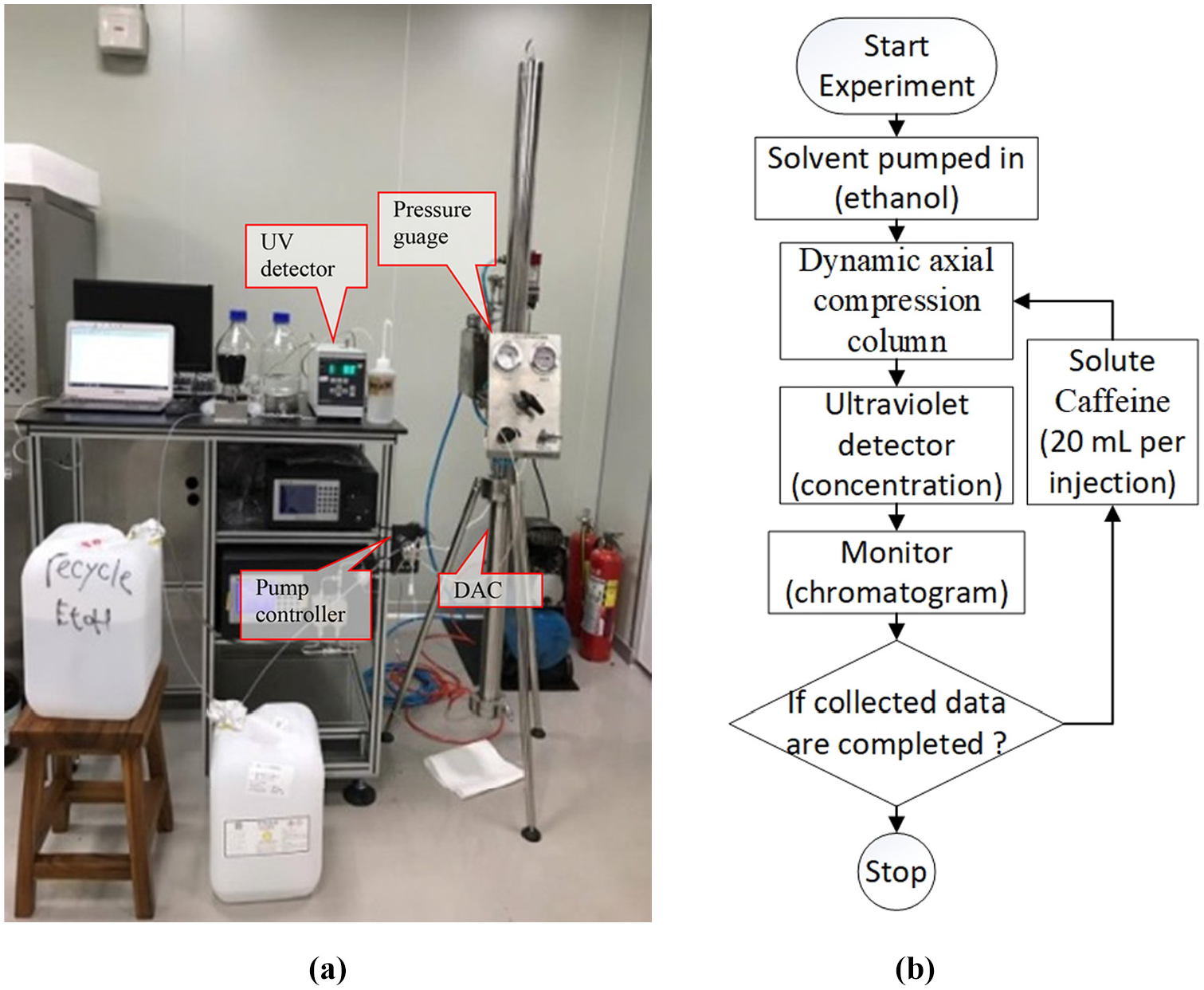
Chromatography experiment: (a) setup and (b) flowchart.

Table 1.

Physical parameters for analysis.

Property	Value	Used in Exp. or CFD
Viscosity	0.0023703 kg m−1 s−1	Exp. and CFD
Density	786 kg m−3	Exp. and CFD
Inlet velocity	0.796 m s−1	Exp. and CFD
Porosity	0.37	Exp. and CFD
Viscous resistance	Frit: 3.5 × 1011 m−2 Packed bed: 3 × 101 m−2	CFD
Pressure	0–200 bar	Exp. and CFD

Exp.: experiment; CFD: computational fluid dynamics.

Mathematical modeling

As shown in Table 1, the inflow Reynolds number (Re) of the present solvent can be calculated to be around one hundred. In addition, the flow Re in the porous zone is 0.1 order of magnitude as expected. Thus, the laminar flow governed the whole flow region of interest, including the channel in the distributor and packed bed. The flow field was described by the transient laminal flow and simulated by the CFD techniques.

Governing equations

The unsteady transport equation of a scalar quantity ϕ is described by the following integral conservation form for an arbitrary control volume V as below ²²

$$\frac{\mathrm{d}}{\mathrm{dt}}\underset{\mathrm{V}}{\int }\rho \varphi \mathrm{dV}+\oint \rho \varphi \overrightarrow{\mathrm{v}}·\mathrm{d}\overrightarrow{\mathrm{A}}=\oint \mathrm{\Gamma }\nabla \varphi ·\mathrm{d}\overrightarrow{\mathrm{A}}+\underset{\mathrm{V}}{\int }{\mathrm{S}}_{\varphi }\mathrm{dV}$$

(1)

where ρ is the density, $\overrightarrow{\mathrm{v}}$ is the velocity vector, $\overrightarrow{\mathrm{A}}$ is the surface area vector, V is the volume, Γ is the diffusion coefficient for ϕ, and S _ϕ is the source term of ϕ per unit volume. Note that ϕ can be replaced by 1 for the continuity equation, and u, v, and w for the momentum equations in the X, Y and Z directions, respectively.

Considering practical situations in the DAC column, the packed bed was simulated by porous medium, which could be modeled by extra source terms including inertial loss and viscous loss (Darcy’s law). The source terms were added to model the porous effect by the following expression

$${\mathrm{S}}_{\mathrm{j}}=-(\frac{\mu }{\alpha }{\mathrm{v}}_{\mathrm{j}}+C\prime \frac{1}{2}\rho \left|\mathrm{v}\right|{\mathrm{v}}_{\mathrm{j}})$$

(2)

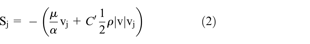
where α indicates the permeability (1/α means viscous resistance), $C\prime$ indicates the inertial resistance factor, and $\left|\mathrm{v}\right|$ is the magnitude of the velocity. Note that the fluid flowed very slowly in the porous zone for the present cases, so the inertial loss (the second term in equation (2)) was neglected to reduce the computing time.

In the present simulations, the injected sample was considered as the pulse input and was numerically treated as the initial and boundary conditions at inlet. At first in simulations, no adsorption between the solute and the stationary phase took place. Therefore, the mass loss between the liquid phase and solid phase could be neglected concerning momentum balance. The species concentration conservation used in present calculations can be described as

$$\frac{\mathrm{d}}{\mathrm{dt}}\underset{\mathrm{V}}{\int }\rho {\mathrm{C}}_{\mathrm{i}}\mathrm{dV}+\oint \rho {\mathrm{C}}_{\mathrm{i}}\overrightarrow{\mathrm{v}}·\mathrm{d}\overrightarrow{\mathrm{A}}=\oint {\mathrm{D}}_{\mathrm{i}}\nabla {\mathrm{C}}_{\mathrm{i}}·\mathrm{d}\overrightarrow{\mathrm{A}}+\underset{\mathrm{V}}{\int }\mathrm{S}\mathrm{dV}$$

(3)

where ${\mathrm{C}}_{\mathrm{i}}$ indicates the mass fraction for species i and ${\mathrm{D}}_{\mathrm{i}}$ is the mass diffusion coefficient for species i in the mixture in the fluid phase.

The adsorption equilibrium has been involved in the packed bed to approach to the practical situations.^23,24 Therefore, the following unsteady term, Q, in differential form was included in the left hand side of equation (3)

$$\mathrm{Q}=\frac{1-\epsilon }{\epsilon }\frac{\partial {\mathrm{q}}_{\mathrm{i}}}{\partial \mathrm{t}}$$

(4)

where ε is the porosity and q_i is the concentration in the solid phase.

Moreover, the linear solid driving force model was used for the component balance in the solid phase

$$\frac{\partial \mathrm{q}}{\partial \mathrm{t}}=\mathrm{k}({\mathrm{q}}^{*}-\mathrm{q})$$

(5)

with q^* = K ${\mathrm{C}}_{\mathrm{i}}$ referring to the concentration in the solid phase in equilibrium with the ${\mathrm{C}}_{\mathrm{i}}$ concentration in the fluid phase, and k indicating the mass transfer coefficient. K is the absorption equilibrium coefficient and was determined by the process of reverse engineering.

The Kozeny–Carman correlation is represented by the following equation ⁸

$$\alpha =\frac{d_p^2·{\epsilon }^2}{150{(1-\epsilon )}^2}$$

(6)

where α is the permeability and d_p is the diameter of packing particles. Equation (6) gives the relation of particle size and porosity. The permeability value can be deduced from CFD and experiments by the process of reverse engineering.

Numerical methods

Since the fluid used in this study is ethanol, the density is assumed to be constant in the present low-speed simulations. By the finite volume method approach, equation (1) is expressed in generalized coordinates for computations. Thus, the discretized formulation for each cell (finite volume) yields

$$\sum _{\mathrm{f}}^{{\mathrm{N}}_{\mathrm{f}}}{\mathrm{v}}_{\mathrm{f}}{\varphi }_{\mathrm{f}}{\mathrm{A}}_{\mathrm{f}}=\sum _{\mathrm{f}}^{{\mathrm{N}}_{\mathrm{f}}}{\mathrm{\Gamma }}_{\varphi }{(\nabla {\varphi }_{\mathrm{f}})}_{\mathrm{n}}{\mathrm{A}}_{\mathrm{f}}+{\mathrm{S}}_{\varphi }\mathrm{V}$$

(7)

where f denotes the face of the finite volume, and N_f is the number of faces enclosing cell.

After combining boundary conditions, equation (7) can be linearized and expressed in the computational domain as

$${\mathrm{a}}_{\mathrm{p}}\varphi =\sum _{\mathrm{nb}}{\mathrm{a}}_{\mathrm{nb}}{\varphi }_{\mathrm{nb}}+\mathrm{b}$$

(8)

where ${\mathrm{a}}_{\mathrm{p}}$ and ${\mathrm{a}}_{\mathrm{nb}}$ are the linearized coefficients for ϕ and ${\varphi }_{\mathrm{nb}}$ and the subscript nb refers to the neighboring cells. The term b is the source term, which includes equation (2) in the porous zone, or the term in equation (4) for treating adsorption equilibrium. The number of neighbors for each finite cell depends on the grid topology but will typically equal the number of faces enclosing the cell. Similar equations can be written for each finite cell in the grid, and this results in a set of algebraic equations to be solved by the SIMPLE algorithm.^25,26

Note that we need to arrange the source term of the governing equations to have negative slope to remedy the convergent problems. Take the term in equation (4) for example; it can be rewritten to be of the following linear form

$$S_{\varnothing }=A+B\varnothing \mathrm{as}\varnothing =c_1,\mathrm{i}=1$$

(9)

$$\{\begin{array}{c}A=\frac{1-\epsilon }{\epsilon }\mathrm{k}·\mathrm{q}\hfill \\ B=-\frac{1-\epsilon }{\epsilon }\mathrm{k}·\mathrm{K}\hfill \end{array}$$

(10)

Hence, we have the negative slope of constant B in equation (10), and that enhances a stable calculation in solving the linearized numerical governing equations of equation (8).

Results and discussions

The results show that CFD combined with CAD solid modeling is a good approach to explore detailed flow fields in DAC columns, and it is an effective method for parameter analysis in innovative distributor design. In addition, the CAD and CFD techniques can provide detailed numerical flows and visualizations. A desktop PC, 32G RAM, quad core, 2.7 GHz CPU, was used to perform the time-marching computation, with a time step of 0.1 s for 60 s, and computation time of 8 h for each case. The convergence criteria for steady or transient numerical calculations were checked by setting the relative residual below 10⁻⁵ for all governing discretized equations. In addition, for transient calculations, the number of inner loop iterations for each calculation step was set to 30. The flow was very slow because of the porous medium inside the DAC column; the inner loop iterations were below 20, obtained from numerical experiments.

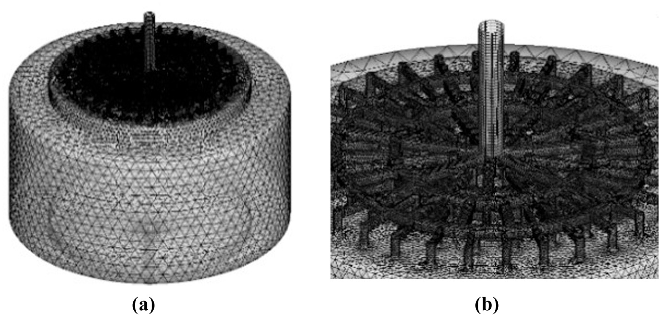
Numerical validations

A model was used for numerical validations based on experimental setups. The mesh was composed of an unstructured grid system with mixed hexahedra and tetrahedral grids. To effectively compute the flow fields, the computational domain was split into smaller subdomains. The mixed grid types were employed to build the mesh around the distributor and frits. Meanwhile, in the packed bed zone, structured hexahedral grids were used to fit the space inside the column. Thus, finer grids were imposed along boundary walls to resolve the laminar boundary layer. The regions near the wall, inlet, and outlet were allocated a slightly higher mesh density as velocity gradient was present. Grid numbers of 0.3, 0.5, 0.8, 1.2, and 1.5 million were selected for grid-independent tests. We found chromatograms were almost indistinguishable for grid numbers over 0.8 million. Therefore, a mesh system of 0.8 million grids was chosen, and simulated results were validated with experiments for our parametric study. Before addressing the flow details, the dominant parameter for CFD, viscous resistance, needs to be determined. Reverse engineering was adopted to determine the unknown value by trial. At the beginning of simulations, a viscous resistance was guessed, and then, the simulated pressure drop between the inlet and the outlet of the column was compared with the experiment data after convergent calculations. By trial and error, the viscous resistance can be determined and used for other parametric studies. Figure 5 compares the pressure drop versus the inlet flow rate. The figure shows that the pressure drop is linearly proportional to the inlet flow rate, and this phenomenon validates Darcy’s law in fluid mechanics. Moreover, the reverse engineering process can also be used to determine the values of the adsorption equilibrium and the mass transfer coefficients.

Figure 5.

Pressure drop versus inlet flow rate.

An advantage of numerical simulation is it provides details about the flow fields, and the corresponding transient flow visualizations can be presented. Figure 6 shows the transient caffeine concentration contours developing in the DAC column with the original 12-opening distributor at various times. At the 60th second, the caffeine concentration is higher at the column header, as depicted by the red color in Figure 6(a). The caffeine then penetrates into the porous zone and diffuses to the whole zone at the 65th second, depicted by the light blue color in Figure 6(b). Eventually, at the 70th second, the caffeine flows out through the exit of the column, and the porous zone is almost occupied by the solvent. Figure 7 shows the corresponding chromatograms of simulation results and experimental data for 200 s. Both chromatograms are normalized by the area under the curves. All simulated values were divided by the peak value. The simulated curve agrees well with the experimental one, and the peak of the CFD curve is a little higher than that of the experiment curve. The minor discrepancy in bandwidths between the simulation and experiment chromatograms shows the dispersion effect in actual situations.

Figure 6.

Flow visualizations on caffeine at various times: (a) 60 s, (b) 65 s, and (c) 70 s.

Figure 7.

The simulated and the experimental chromatograms.

New distributors

The new distributor designed by method 1 is displayed by solid modeling (Figure 8) and has been patented by the Taiwanese government. ²¹ The distributor was created as a two-disk compound, which can accommodate more openings without violating the proposed rules in the present design procedure. There are 96 openings on the distributor compound, as shown in Figure 8(b), with 48 openings on the upper disk and 48 openings on the bottom disk. As compared with the column, the sizes of openings and channels on the disk surfaces are relatively small. Thus, the grids around these regions need to be finer to resolve the flow fields as shown in Figure 9. Figure 9 displays the grid system for the new distributor. The total grid number is around 0.8 million in Figure 9(a), while the detailed allocation of the grid system is shown in Figure 9(b). Figure 10 illustrates the simulated flow by CFD for the new distributor with pressure contours in Figure 10(a) and path lines in the flow in Figure 10(b).

Figure 8.

New 96-opening distributor designed by method 1: (a) upper disk, (b) bottom disk and (c) the compound.

Figure 9.

Grids for the new distributor: (a) 0.8 million grids and (b) detailed grid allocation.

Figure 10.

Numerical illustrations for the new distributor: (a) pressure contours and (b) path lines in the flow.

Figure 11 shows the axial velocity profiles from numerical simulations at the inlet of the porous zone without a distributor installed. The flow appears to be of peak shape around the column center due to the small opening of the feeding pipe at the column header. The distributor nevertheless can play a key role to make the flow even, as demonstrated in Figure 12. Figure 12 illustrates the velocity profiles when the 12-opening original distributor is used (velocity magnitude presented by red square dots), and the new 96-opening distributor (profile presented by the blue line). To show the benefit of installing the distributor, the velocity profiles were evaluated in terms of the average velocity deviation, which indicates the deviated value from the average velocity at the column cross-section. The average velocity deviation was evaluated to be 1.598e−3 m s⁻¹ from Figure 11, and the figure shows that the flow velocity profile was uneven. The average velocity deviation for the column with the new 96-opening distributor was 8.451e−5 m s⁻¹ (Figure 12), while that for the column with the conventional 12-opening distributor was 5.689e−4 m s⁻¹, which indicates that the flow profile at the porous zone inlet with the new distributor was more uniform than that with the commercial distributor.

Figure 11.

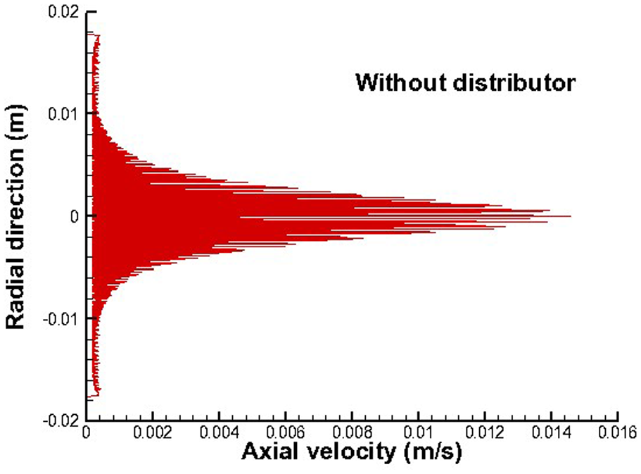
Velocity profile at the inlet of porous zone without a distributor.

Figure 12.

Velocity profiles by two designs at the exit of distributor.

The previous calculations did not include the additional equations with adsorption equilibrium, and consequently, the actual flow field in the porous zone could not be satisfactorily simulated. To reduce the difference between the simulation result and the actual condition, extra programs were written and were coupled with the original Fluent to simulate the interaction of the solute and particles in the packed bed, that is, absorption and precipitation. As mentioned previously, reverse engineering can be applied to determine the value of the adsorption equilibrium and the mass transfer coefficients. Thus, the originally unknown adsorption equilibrium coefficient of K was selected to be 0.1, and the mass transfer coefficient was set to be 0.05 as the adsorption separation process was activated. The numerical and experimental results are compared in Figure 13. There are two lines representing the numerical simulations; the dashed line is the chromatogram without considering adsorption, while the solid one is that with adsorption considered. The peak of the dashed line is higher than that of the solid one and features no significant tailing. However, the simulated chromatogram with adsorption is closer to the experimental result. Therefore, it is more practical to simulate the flow field in the DAC column while considering the interaction between the mobile phase and the solid phase.

Figure 13.

Comparisons of experiment and CFD with adsorption considered.

Conclusion

High-performance distributors are essential for the preparative DAC columns with low length-to-diameter ratio. In this study, we propose a design procedure for new distributors. The vital characteristics of the chromatography process were simulated by the CFD and validated by experiments for the new 96-opening distributor. Moreover, originally unknown numerical parameters, such as viscous resistance and adsorption coefficients, were effectively determined by reverse engineering. The 96-opening distributors were investigated numerically and experimentally, and both results demonstrated that they outperformed the commercial distributors. Moreover, the flow profile at the porous zone inlet with the new distributor was more uniform than that with the commercial one. Including the adsorption equilibrium in the traditional governing equations made the measurement data closer to the chromatogram curve. Therefore, the adsorption process should be included in future works for practical applications.