Quasi-analytical solutions of a turbulence-modeling equation on the robustness of decaying homogeneous turbulence

Abstract

The present study introduces third-order quasi-analytical solutions of a turbulence-modeling equation, where the standard $k-ϵ$ model equation is used because this model is commonly and widely used in engineering applications. These quasi-analytical solutions describe the robustness of decaying homogeneous turbulence. In the present study, decaying homogeneous turbulence influenced by a weak fluid acceleration of mean flow, which is equivalent to the small strain of the mean flow, is considered. Here, the small strain of the mean flow only slightly affects the anisotropy of the decaying homogeneous turbulence, as shown in previous experiments. Simplified governing equations are derived from the governing equations of the turbulence modeling by introducing the conditions of the small strain. Here, two nondimensional functions are introduced in order to describe the influence on the turbulent kinetic energy and its dissipation using decay laws of the turbulent kinetic energy and its dissipation. Three constants included in the quasi-analytical solutions could be obtained using observable parameters.

Introduction

Fluid flow in turbulence is widely found in fluid-engineering applications. Homogeneous turbulence, which is accompanied by the production of kinetic energy due to the mean shear, decays as time proceeds. Turbulent kinetic energy k in the decaying homogeneous turbulence has been extensively studied, both experimentally and theoretically. In wind tunnel experiments, grid-generated turbulence is equivalent to decaying homogeneous turbulence. The decay power law of turbulent kinetic energy ¹ is used to derive the basis of turbulence models, such as the standard $k-ϵ$ model. Here, decay exponent n is included in the decay power law of turbulent kinetic energy. The value of the decay exponent n has also been investigated in previous studies. ² In high-Reynolds-number grid-generated turbulence, the value of the decay exponent may approach that of Saffman turbulence. ³ Direct numerical simulation (DNS) is also used to study the grid-generated turbulence. ⁴

For decades, numerous studies have investigated and summarized the results of decaying homogeneous turbulence.^5–7 DNS has significantly contributed to investigating the characteristics of decaying homogeneous turbulence.^8–10 The turbulent Reynolds number, which can be set, had been critically limited to be low in previous DNS studies. Then, it has become possible to analyze homogeneous turbulence at sufficiently high Reynolds numbers. ¹¹ These DNS studies are mainly performed using the Fourier spectrum method. ¹² Our study considers that one of the significant contributions of using DNS in the study of homogeneous turbulence is the numerous investigations of small-scale turbulence characteristics. ¹³ Knowledge of small-scale turbulence characteristics is also essential from the viewpoint of turbulence modeling using large-eddy simulation. Decaying homogeneous turbulence can correspond to grid-generated turbulence in experimental studies. Grid-generated turbulence is generated using a turbulence-generating grid and has been experimentally investigated in many previous studies.^{1–3,14–17} Previous DNS studies have also considered grid-generated turbulence used in previous experimental studies.^18–20 In our study, the effects of very weak fluid acceleration of the mean flow on decaying homogeneous turbulence are considered. An example of a summary of the effects of mean fluid acceleration on homogeneous turbulence has been shown in a previous study. ⁶

The standard $k-ϵ$ model is commonly and widely used as the simplest complete turbulence model in fluid-engineering applications. In the standard $k-ϵ$ model, the decay exponent derives the value of the model constant. ¹⁰ The value of the decay exponent included in the decay law of the turbulent kinetic energy is essential in the application of the turbulence model. The decay exponent is important in order to quantify the decay characteristics of decaying homogeneous turbulence, or grid-generated turbulence. At low to moderate Reynolds numbers, previous experiments did not come to a consensus regarding the value of the decay exponent in the decaying homogeneous turbulence. In the range of moderate Reynolds numbers, there could be a significant dispersion of the decay exponent.^21,22 Factors that affect the decay characteristics of the homogeneous turbulence have been studied in previous studies. There may be potential effects of the initial condition on the decaying characteristics. The difference in the initial flow field may significantly affect values of the decay exponent.^14,15,23 Recently, grid-generated turbulence, which is generated by a multiscale-generated grid, has been investigated.^24–28 The multiscale generation of turbulence may affect the dissipation of the decaying homogeneous turbulence.^29,30 In addition, the effects on the large-scale structure of decaying turbulence could affect the decay characteristics of homogeneous turbulence. ³¹

The present study considers the sensitivity of decaying homogeneous turbulence, especially turbulent kinetic energy in the turbulence, to small influences due to the mean flow based on several previous studies. The acceleration of the free stream is used as the source influencing decaying homogeneous turbulence. The acceleration of the free stream, which is equivalent to the strain of the mean flow, is a factor that could affect the decay characteristics of homogeneous turbulence. The decay characteristics of homogeneous turbulence are rather sensitive to the acceleration of the free stream, even if the acceleration of the free stream is weak. ¹⁴ As shown in a recent study measuring grid-generated turbulence, ¹⁶ the weak fluid acceleration, which only slightly affects the anisotropy of grid-generated turbulence, ³² may reduce the turbulent kinetic energy in grid-generated turbulence. In an actual experimental situation, this weak fluid acceleration could be caused by the blockage of a wind tunnel.^33,34 Few previous studies examined the effects of the weak fluid acceleration,^17,35,36 the small strain of the mean flow, due to wind tunnel blockage of the grid-generated turbulence, whereas there are several previous studies that examined the effects of wind tunnel blockage on the flow around an obstacle or a wind turbine.^37–41 In a recent experiment on grid-generated turbulence using a wind tunnel, the blockage effects, which may be equivalent to the effects of weak fluid acceleration, were confirmed to be negligible. ¹⁷

The purpose of the present study is to derive quasi-analytical solutions of the turbulence-model equations in order to specify the sensitivity of decaying homogeneous turbulence, which describes the effects of the small strain on the decaying homogeneous turbulence. The standard $k-ϵ$ model is considered in the present study because this model is widely and commonly used in engineering applications. In the present study, mathematical solutions in the temporal region, in which relative effects of the small strain are greater than 1%, are derived. In addition, based on a previous study, we examine two variations of the small strain in the present study, which are a constant variation or a linear variation with respect to time. ³⁶

The remainder of the present article is organized as follows. First, the governing equations and numerical conditions are shown in “Methods” section. In this section, the governing equations are derived from the standard $k-ϵ$ model equation using the decay laws of the turbulent kinetic energy and its dissipation. In addition, the two temporal variations of the small strain are described in detail. Then, the results and a discussion are presented. The quasi-analytical solutions are derived and validated using the present numerical results. In addition, the derived analytical solutions are discussed based on constants included in the derived solutions, as well as previous studies. Finally, the findings of the present study are summarized. We believe that the innovative point of our study is that a mathematical solution of the $k-ϵ$ model, which is a quite general model, has been derived. The mathematical solution of the $k-ϵ$ model, which can be derived here, can allow us to understand the characteristics of the general model. This mathematical model will be able to be improved using the mathematical solution of the model. Moreover, this mathematical solution has been obtained by approaching the robustness of decaying turbulence, which is widely found in fluid-engineering applications.

Methods

Governing equation

In the present study, decaying homogeneous turbulence affected by the small strain of the mean flow was investigated. Here, the present decaying homogeneous turbulence has axisymmetric anisotropy, similar to that of grid-generated turbulence. ¹ In addition, the present study focuses on the small strain, which does not affect the anisotropy of the decaying homogeneous turbulence, as reported in a previous experiment.^16,17 We studied the response of decaying homogeneous turbulence with axisymmetric anisotropy to a very weak acceleration of the mean flow. In general, the acceleration of the mean flow affects the anisotropy of the turbulence.^6,32 In the results of previous studies, we can see results whereby the value of the anisotropy of decaying homogeneous turbulence changes only slightly in the streamwise direction when the acceleration of the mean flow is very weak.^16,32 As seen in previous studies, even if the anisotropy changes in the streamwise direction due to large total strain, the anisotropy is considered to change little in the region of very small total strain. The acceleration of the mean flow is set to be very weak so as not to affect the anisotropy of the decaying homogeneous turbulence. The mean flow of decaying homogeneous turbulence with axisymmetric anisotropy is ideally constant. We examine the robustness of decaying homogeneous turbulence by considering the condition in which the mean flow acceleration is very weak. An important assumption is made whereby the very weak acceleration of the mean flow does not affect the anisotropy. Although this may not be a weak assumption, quasi-analytical solutions could be derived using this assumption. The small acceleration of the mean flow observed reduces the turbulent energy, which is qualitatively consistent with the results of previous wind tunnel experiments.^16,32

For the decaying homogeneous turbulence used in the present study, the governing equations of the standard $k-ϵ$ modeling are as follows ¹⁰

$$\frac{dk}{d{t}^{\prime }}=P-ϵ\mathrm{and}\frac{dϵ}{d{t}^{\prime }}=C_{ϵ1}P\frac{ϵ}{k}-C_{ϵ2}\frac{{ϵ}^2}{k}$$

(1)

where $k(=(1/2)(〈u^2〉+〈v^2〉+〈w^2〉))$ is the turbulent kinetic energy; u, v, and w are the velocity fluctuations in the streamwise, transverse, and spanwise directions, respectively; and $〈〉$ denotes the ensemble average. In the governing equations, $ϵ$ is the dissipation of the turbulent kinetic energy, and $t\prime$ is the dimensional time. Moreover, $C_{ϵ1}$ is the model coefficient, and the other model coefficient $C_{ϵ2}$ ¹⁰ is described as $C_{ϵ2}=(n+1)/n$ . Using the axisymmetric anisotropy of the homogeneous turbulence, the term P is the production term and is given as $P=(1/2)(-2〈u^2〉+〈v^2〉+〈w^2〉)(\mathrm{dU}/\mathrm{dx})$ ,^17,35 where $\mathrm{dU}/\mathrm{dx}$ is the longitudinal gradient of the streamwise mean velocity U, and x is the streamwise direction. Previous studies of grid-generated turbulence ¹ used the anisotropy parameter a, which is defined as follows: $a=〈v^2〉/〈u^2〉=〈w^2〉/〈u^2〉$ . Using the anisotropy parameter a, the production term P results in the following form

$$P=P_o\frac{\mathrm{dU}}{\mathrm{dx}}k(t\prime ),\mathrm{where}{P}_o=\frac{2(a-1)}{1+2a}$$

(2)

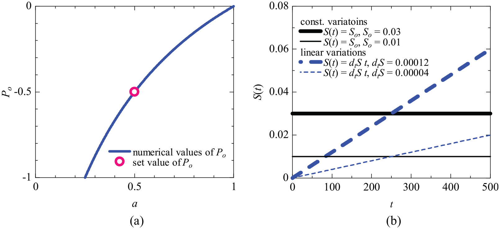
Figure 1(a) shows the magnitude of the production term $P_o$ as a function of the anisotropy a. As shown in the figure, the enhancement of the anisotropy, described as the deviation of a from unity, increases the absolute value of $P_o$ . In general, mean fluid acceleration significantly affects anisotropy, as shown in previous studies.^6,32 On the other hand, as seen in previous studies,^16,32 there is a condition whereby the acceleration of the mean flow is very weak and has little effect on the anisotropy of the decaying homogeneous turbulence. In our study, we consider the acceleration of the mean flow, which only slightly affects the anisotropy as a very weak acceleration. In other words, the change of anisotropy due to the very weak fluid acceleration is on the order of uncertainty of the experiment. Using this very weak mean flow acceleration, the robustness of decaying homogeneous turbulence is investigated. As seen in turbulence textbooks,^6,7 there are three stages for grid-generated turbulence. This study focuses on the second stage, in which fully developed decaying homogeneous turbulence exists. At this stage, the turbulent kinetic energy and its dissipation rate are described by each power law. The turbulent Reynolds number of the decaying homogeneous turbulence assumed in our study is assumed to be sufficiently high to use the standard $k-ϵ$ model.

Figure 1.

(a) Profile of $P_o$ as a function of the anisotropy a by equation (2). The present setting of $P_o$ is shown by the open circle. (b) Examples of temporal profiles of the small mean strain $S(t)$ , where $S(t)=S_o$ or $S(t)=d_t\mathrm{St}$ . Here, $S_o=0.01$ or $0.03$ , and $d_{t}S=0.00004$ or $0.00012$ . Note that the value of $d_{t}S$ could be related to that of $S_o$ . These values of $d_{t}S$ are set using equation (6) from $S_o$ .

In the decaying homogeneous turbulence which is not affected by the small mean strain, the turbulent kinetic energy k and its dissipation $ϵ$ could be described, respectively, by the following decay laws

$$k(t)=k_o{t}^{-n}\mathrm{and}ϵ(t)={ϵ}_o{t}^{-(n+1)}$$

(3)

where $k_o=k(1)$ , ${ϵ}_o=n(U_o/M)k_o$ , $t=t\prime /t{\prime }_o$ , and $t{\prime }_o=M/U_o$ . Here, M and $U_o$ are the mesh size of a turbulence-generating grid and the inflow streamwise mean velocity, respectively, which are the characteristic length and the characteristic velocity, respectively. in addition, $k_o$ could be referred to as the decay coefficient. ² In the decay laws, n is the decay exponent and is on the order of unity. The value of the decay exponent quantifies the decay characteristics of the decaying turbulence and has been measured in previous studies.^{1–3,14–17,21,22,26} In addition, the value of n may depend slightly on the turbulent Reynolds number. In the lower Reynolds number range, the value of the decay exponent could be increased.^16,22,42 In the present study, the decay laws are used to examine the effects of the small mean strain on the decaying homogeneous turbulence. The present study introduces the influence functions $f(t)$ and $g(t)$ , which are defined as follows

$$k(t)=f(t)k_o{t}^{-n}\mathrm{and}ϵ(t)=g(t){ϵ}_o{t}^{-(n+1)}$$

(4)

The influence functions describe the relative effects of the small mean strain on the turbulent kinetic energy and its dissipation. When the small strain is absent, the influence functions are unity: $f(t)=1$ and $g(t)=1$ .

Then, governing equations of the influence functions $f(t)$ and $g(t)$ will be derived. In the present study, the governing equations of the turbulent kinetic energy and its dissipation are given as equations (1) and (2). In addition, as shown in equation (4), we have introduced the influence functions $f(t)$ and $g(t)$ to characterize the turbulent kinetic energy and its dissipation in the decaying homogeneous turbulence sensitized to the small strain. Using equations (1), (2), and (4), the governing equations of the influence functions could be derived as follows

$$\begin{array}{c}\frac{\mathrm{df}(t)}{\mathrm{dt}}=P_{o}S(t)f(t)+n\frac{f(t)-g(t)}{t}\mathrm{and}\hfill \\ \frac{\mathrm{dg}(t)}{\mathrm{dt}}=C_{ϵ1}{P}_{o}S(t)g(t)+(n+1)\frac{g(t)}{f(t)}\frac{f(t)-g(t)}{t}\hfill \end{array}$$

(5)

Note that these governing equations do not include the decay coefficients $k_o$ and ${ϵ}_o$ . The turbulence intensity and the turbulent Reynolds numbers of the decaying homogeneous turbulence depend on the decay coefficients in the initial time. Therefore, for various initial values of the turbulence intensity and the turbulent Reynolds numbers, analytical solutions of the derived governing equations could be derived. The governing equations include the decay exponent n, which could depend on the Reynolds number.^16,22,42 In the present governing equations, the Reynolds number dependency of $f(t)$ and $g(t)$ can be described using the decay exponent n.

Numerical condition

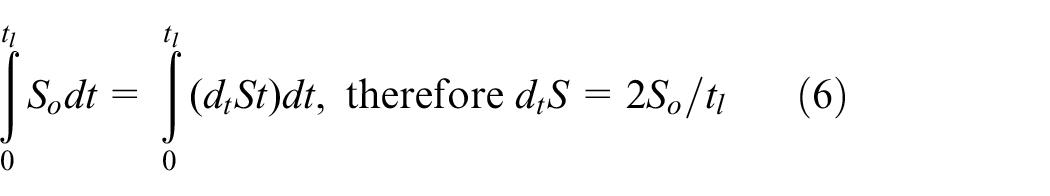
In the governing equations, the small strain $S(t)$ is included, which is a function of the time t. A temporal variation of $S(t)$ should be given in order to solve the governing equations. The present study used two temporal variations of $S(t)$ . The first temporal variation is a constant variation. In this case, temporal variations of $S(t)$ are given as follows: $S(t)=S_o$ . This constant variation is the same as that used in previous studies.^17,35 The second temporal variation is a linear variation. The linear variation of $S(t)$ is given as follows: $S(t)=d_t\mathrm{St}$ , where $d_{t}S$ is a linear gradient of the variations. The values of $S_o$ and $d_{t}S$ should be set to solve the governing equations. For setting a value of $S_o$ and $d_{t}S$ , the present study uses the following relation between $S_o$ and $d_{t}S$

$$\underset{0}{\overset{t_l}{\int }}{S}_o\mathrm{dt}=\underset{0}{\overset{t_l}{\int }}(d_t\mathrm{St})\mathrm{dt},\mathrm{therefore}{d}_{t}S=2S_o/t_l$$

(6)

Here, $t_l$ is the integral range of t, and, in the present study, $t_l$ is set to $t_l=500$ . Figure 1(b) shows the constant and linear variations of $S(t)$ schematically. Here, in the figure, the values of $S_o$ are set to be $S_o=0.03$ and $S_o=0.01$ . Using $t_l=500$ , two values of $d_{t}S$ are derived using equation (6) as $d_{t}S=0.00012$ and $d_{t}S=0.00004$ for $S_o=0.03$ and $S_o=0.01$ , respectively.

The present numerical conditions are shown as follows. The governing equations are numerically solved from $t=0$ to $t=500$ . The small strain $S(t)$ is set as the constant variation or linear variation, as shown above. The constant $S_o$ in the constant variation is varied as $S_o=0.03$ , $0.01$ , $0.003$ , and $0.001$ . In the present study, $t_l=500$ is used to calculate values of $d_{t}S$ using equation (6). Note that condition $t_l=500$ is equivalent to $x/M=500$ with zero magnitude of the small strain. The values of $d_{t}S$ in the linear variation are varied based on these values of $S_o$ as $0.00012$ , $0.00004$ , $0.000012$ , and $0.000004$ . The coefficient $P_o$ is included in the governing equations and depends only on the anisotropy a, as shown in equation (2). The value of the anisotropy parameter a is set to $a=0.5$ based on previous experiments.^1,2 Here, the anisotropy of the grid-generated turbulence is considered to be constant for the streamwise direction based on a previous experiment. ¹⁶ The present value of $P_o$ is given as $P_o=-0.5$ using $a=0.5$ . These values of $P_o$ and a are shown in Figure 1(a). The model coefficient $C_{ϵ1}$ is set to $C_{ϵ1}=1.44$ . This value could be one of the most widely used for $C_{ϵ1}$ . ¹⁰ The decay exponent n is set to $n=1.2$ , which may be a notable value in the grid-generated turbulence shown in previous studies. ³ This value of the decay exponent has been investigated as the typical value of the high-Reynolds-number grid-generated turbulence. ²² Although we are interested in the effect of the magnitude of anisotropy, we do not consider this effect in our study. The use of the standard $k-ϵ$ model enables us to derive quasi-analytical solutions. The parameter a representing anisotropy is simply a coefficient that describes the magnitude of the product term in the governing equations, as shown in equation (2). This coefficient changes directly for anisotropy a, as shown in Figure 1(a). This coefficient is also included in the derived quasi-analytical solutions. Therefore, the value of anisotropy parameter a does not affect the mathematical form of the obtained quasi-analytical solutions.

Results and discussion

Numerical results

The purpose of the present study is to find analytical solutions that satisfy the governing equations of the influence functions. Thus, the present study looks anew at the forms of the governing equations (equation (5)). In both of the governing equations, the term $(f(t)-g(t))/t$ is included. Thus, similar to a previous study, the present study focuses on this term to solve the governing equation. ¹⁷ Here, the previous study solved the governing equation mathematically by forming the term $(f(t)-g(t))/t$ using methods of numerical simulation. A function of time $h(t)$ , which is defined as follows, is used

$$h(t)=\frac{f(t)-g(t)}{t}$$

(7)

Figure 2(a) shows temporal profiles of the form $h(t)$ for constant and linear variations of the small strain. As shown in the figure, a temporal profile depends on the variation of the small strain, as well as the magnitudes of the strain. For constant variations of the small strain, the value of $h(t)$ is decreased as the nondimensional time increases. For linear variations, the temporal profiles could have a value of the local maximum. In a sufficiently large nondimensional time, the value of $h(t)$ may decrease as the nondimensional time increases.

Figure 2.

(a) Temporal variations of $h(t)$ as a function of t, where $h(t)$ is a key part included in the governing equation. Temporal variations of $h(t)$ depend on the shape of the variation, as well as the magnitude of the small strain. (b) Based on the total strain $\sigma (t)$ (equation (8)) and $S(t)$ , the temporal variations of $h(t)/S(t)$ collapsed.

As shown in Figure 2(a), the temporal profile of $h(t)$ could depend on the magnitude of the small strain, as well as a temporal variation of the small strain. Note that, in the present study, the dependency of the term on the magnitude of the small strain may be reduced. In order to reduce this dependency, the present study uses total strain which, similar to a previous study, ³⁶ is defined as follows

$$\begin{array}{c}\sigma (t)=\underset{0}{\overset{t}{\int }}{S}_o\tau d\tau =S_{o}t\mathrm{or}\hfill \\ \sigma (t)=\underset{0}{\overset{t}{\int }}{d}_{t}S\tau d\tau =\frac{1}{2}{d}_{t}S{t}^2\hfill \end{array}$$

(8)

Here, the total strain $\sigma (t)$ is described as the temporal integrals of each small strains. Figure 2(b) shows the temporal profiles of $h(t)$ using the total strain, where the function value is taken to be $h(t)/S(t)$ , rather than $h(t)$ itself. As shown in Figure 2(b), the independence of the magnitude of the small strain could be given using the total strain, as well as $h(t)/S(t)$ . Thus, $h(t)/S(t)$ is considered to decrease as the total strain $\sigma (t)$ increases. As shown in Figure 2(b), the temporal profile of $h(t)/S(t)$ depends precisely on the temporal variation of the small strain. In addition, $h(t)/S(t)$ with the constant variations of the small strain is more significant than that with the linear variations.

Quasi-analytical solutions

The present study uses $h(t)$ included in the governing equations to solve the equations analytically. The governing equation of the influence function of the turbulent kinetic energy $f(t)$ can be analytically solved by forming $h(t)$ in the first step. An analytical solution of the other influence function $g(t)$ can also be derived using both the form of $h(t)$ and the derived solution of $f(t)$ . Few previous studies also focus on forming $h(t)$ to solve the governing equations ¹⁷ describing $h(t)$ as a constant variation of time, where the constant variation includes the magnitude of the small strain. In addition, a subsequent study used an exponential function and a linear function of time to approximate $h(t)$ . In these studies, the small strain is taken to be a constant of time.

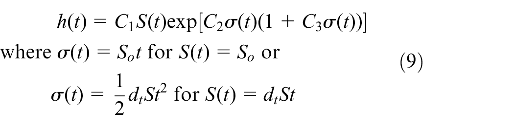
The present study uses the following function to approximate the temporal profiles of $h(t)$

$$\begin{array}{c}h(t)=C_{1}S(t)\exp [C_2\sigma (t)(1+C_3\sigma (t))]\hfill \\ \mathrm{where}\sigma (t)=S_{o}t\mathrm{for}S(t)=S_o\mathrm{or}\hfill \\ \sigma (t)=\frac{1}{2}{d}_{t}S{t}^2\mathrm{for}S(t)=d_t\mathrm{St}\hfill \end{array}$$

(9)

Here $C_1$ , $C_2$ , and $C_3$ are constants. The values of the constants are calculated in order to approximate the temporal profiles of $h(t)$ by equation (9). Figure 3(a) shows the temporal profiles of the above approximation, which are fitted to each temporal profile of $h(t)$ . As shown in the figure, equation (9) could approximate the temporal profiles of $h(t)$ with sufficient accuracy. Figure 3(b) shows the observed values of the constants, which are calculated to fit the temporal profiles. As shown in the figure, the values of the constants depend on the temporal variation of the small strain. Note that the dependency of $h(t)$ on the temporal variations of the small strain is described by that of the constants. The effects of a nonzero value of $C_3$ may not be negligible in the approximation, although the absolute value of $C_3$ is smaller than that of $C_1$ and $C_2$ . As shown in Figure 3(a), the approximation of $h(t)$ with zero value of $C_3$ deviates from the numerical results in the range of large $\sigma (t)$ .

Figure 3.

(a) Temporal profiles of $h(t)/S(t)$ approximated by the present form of $h(t)$ (equation (9)), which could approximate well the numerical results. Note that the effects of $C_3$ on the accuracy of the approximation were not negligible. The effects of $C_3$ on the accuracy of the approximation, shown as the deviation from the numerical values, are increased as the total strain $\sigma (t)$ increases. Here, the mathematical form that can approximate the numerical results is significantly limited. For instance, a quadratic form, the number of coefficients to be calculated for which is the same as that of the present form, could fail to approximate the numerical results shown in (b). The observed value of $h(t)/S(t)$ could depend on the small strain variation $S(t)$ , as shown in (a). (b) This dependency is found to be equivalent to the difference in the coefficient values between the variations.

The present study used a function based on an exponential function, as shown in equation (9), to approximate temporal profiles of $h(t)$ . Conceivably, only the equation may approximate $h(t)$ with sufficient accuracy. In order to discuss this issue, the present focuses on the number of constants included in the approximation. The present approximation equation (9) includes three constants, $C_1$ , $C_2$ , and $C_3$ . For instance, the present study examines a quadratic function, which is a function with three constants, $h(t)=C_1+C_{2}t+C_3{t}^2$ , for the approximation. However, as shown in Figure 3(a), a quadratic function fitted to the temporal profiles of $h(t)$ allows significant deviation from the numerical results. The quadratic function was not suitable to approximate the temporal profiles of $h(t)$ with sufficient accuracy. Thus, this result suggests that several constants would be required to approximate $h(t)$ when a polynomial equation is used for the approximation. In contrast to the quadratic approximation, the present approximation (equation (9)) uses only three constants to approximate the temporal profiles of $h(t)$ .

For the constant variation of the small strain, the governing equation of $f(t)$ yields the following equation, using equation (9) for $h(t)$

$$\frac{\mathrm{df}(t)}{\mathrm{dt}}=P_o{S}_{o}f(t)+n{C}_1{S}_o\exp [C_2{S}_{o}t(1+C_3{S}_{o}t)]$$

(10)

The derived governing equation may be solved analytically. The analytical solution of the derived governing equation is derived as follows

$$\begin{array}{c}\multicolumn{1}{c}{f(t)=\exp \left(P_o{S}_{o}t\right)}\\ \times (\frac{1}{2}\sqrt{\frac{\pi }{-C_2{C}_3}}n{C}_1\exp \left(\frac{{(C_2-P_o)}^2}{4C_2{C}_3}\right)\hfill \\ \times \mathrm{erf}\left(\frac{P_o-C_2(1+2C_3{S}_{o}t)}{2\sqrt{-C_2{C}_3}}\right)+C_o)\hfill \end{array}$$

(11)

Here, $C_o$ is an integral constant. In addition, $-C_2{C}_3$ is positive, as shown in Figure 3(b). The mathematical form of the above analytical solution is not sufficiently simple, although the above solution is derived as an analytical solution of the governing equation. Note that the error function is included in the analytical solution of equation (11). Therefore, the above analytical solution may not be suitable to calculate a value of $f(t)$ directly. Moreover, the previous analytical solutions of $f(t)$ ^17,35 are based on an exponential function and differ significantly from the above analytical solution. Thus, the above analytical solution may not be discussed using the previous analytical solutions.

The present study attempts to derive an analytical solution for $f(t)$ other than the analytical solution of equation (11), rewriting the approximation of $h(t)$ (equation (9)) as follows: $h(t)=C_{1}S(t)\exp (C_2\sigma (t)+C_2{C}_3\sigma (t{)}^2)$ . Then, the present study focuses on the numerical results whereby the value of $C_2{C}_3$ is small, as shown in Figure 3(b). When the value of $C_2{C}_3$ is sufficiently small, the approximation of $h(t)$ could result in the following form

$$h(t)=C_{1}S(t)(1+C_2{C}_3\sigma (t{)}^2)\exp (C_2\sigma (t))$$

(12)

Here, note that a variable of the exponential function is changed to $C_2\sigma (t)$ from $C_2\sigma (t)(1+C_3\sigma (t))$ . The governing equation of $f(t)$ using the refined approximation could also be analytically solved as equation (13) in the next page. As shown in the above equation, the refined analytical solution of $f(t)$ does not include the error function and is significantly simplified. In addition, this refined analytical solution could be discussed using the previous analytical solutions.^17,35 Thus, the present study uses the refined analytical solution of equation (13). An analytical solution of $g(t)$ can also be obtained from $f(t)$ using the approximation of $h(t)$

$$\begin{array}{c}\multicolumn{1}{c}{f(t)=\exp (P_o\sigma (t))-\frac{n{C}_1(C_2(C_2+2C_3)-P_o(2C_2-P_o))}{{(C_2-P_o)}^3}\exp (P_o\sigma (t))}\\ +n{C}_1\frac{{(C_2-P_o)}^2+C_2{C}_3[{(1+P_o\sigma (t))}^2+{(1-C_2\sigma (t))}^2-2P_o{C}_2\sigma {(t)}^2]}{{(C_2-P_o)}^3}\exp (C_2\sigma (t))\hfill \end{array}$$

(13)

$$\begin{array}{c}\multicolumn{1}{c}{(\mathrm{LHS})=[P_o(n-1)C_1]S_o}\\ +[P_o(n{C}_1+P_o)+(n-2)C_1{C}_2]S_o\sigma (t)\hfill \\ +(1/2)[P_o^2(n{C}_1+P_o)\hfill \\ +C_1{C}_2(n{P}_o+(n-3)(C_2+2C_3))]S_o\sigma (t{)}^2+\cdots \hfill \end{array}$$

(14)

$$\begin{array}{c}\multicolumn{1}{c}{(\mathrm{RHS})=[(n+1)C_1+C_1{P}_o]S_o}\\ +[(n+1)C_1(C_2-C_1)\hfill \\ +C_1{P}_o(C_1(n-1)+P_o)]S_o\sigma (t)\hfill \\ +(1/2)[(n+1)C_1{C}_2(C_2+2C_3-4C_1)\hfill \\ +2(n+1)C_1^2(n{C}_1+P_o)\hfill \\ +P_o[C_1((n-2)C_1{C}_2\hfill \\ +(n{C}_1+P_o))]]S_o\sigma (t{)}^2+\cdots \hfill \end{array}$$

(15)

The form by which to approximate $h(t)$ is determined from the viewpoint of applied mathematics. As shown in equation (5), $\mathrm{nh}(t)$ , the second term of $f(t)$ , corresponds to the inhomogeneous term of the ordinary differential equations (ODE). We consider that the derived form of quasi-analytical solutions should be as mathematically simple as possible. The selected mathematical form to describe the inhomogeneous term directly affects the form of the derived quasi-analytical solutions. Typically, a general analytical solution of an ODE, including an inhomogeneous term, is given based on the exponential function. Therefore, we consider that the inhomogeneous term based on the exp function would simplify the form of the quasi-analytical solutions. In fact, by setting the inhomogeneous term as equation (12), equation (13) can be derived as a quasi-analytical solution as a simple form. The validity of giving the inhomogeneous term based on the exp function is considered in the results of the present numerical analysis. As shown in Figure 3(a), the primary part of the inhomogeneous term, $h(t)$ , can be appropriately approximated using a function based on the exp function. The primary part $h(t)$ can be approximated using only three constants. If polynomials or logarithmic functions are used to approximate $h(t)$ , more constants must be included. We consider the results of approximating $h(t)$ with three constants that are needed to know if the number of the constants sufficient to approximate $h(t)$ is two. In our study, $h(t)$ is approximated using three constants, and the necessity of the third constant $C_3$ is considered and discussed.

The derived solution of $f(t)$ (equation (13)) includes the constants $C_1$ , $C_2$ , and $C_3$ . The forms that describe these constants should be derived. The present study should use the governing equation of $g(t)$ as well as that of $f(t)$ for analysis. Thus, in the present study, the governing equation of $g(t)$ is used to derive the forms of these constants. The forms of these constants for constant variation of the small strain are first examined. The solution of $g(t)$ could be derived from the analytical solution of $f(t)$ using equation (9). For the constant variation of the small strain, the left-hand and right-hand sides (LHS and RHS) of the governing equation of $g(t)$ can be derived as equations (14) and (15), where we focus on the small magnitude of $S_o$ . Since the LHS is equal to the RHS, the forms of the constants could be derived as follows

$$\begin{array}{c}{C}_1=-\frac{C_{ϵ1}-1}{2}{P}_o\hfill \\ C_2=-\frac{3n(C_{ϵ1}-1)-(C_{ϵ1}+5)}{6}{P}_o,\mathrm{and}\hfill \\ C_3=\frac{1}{12}\frac{{(C_{ϵ1}-1)}^2(3n+1)}{3n(C_{ϵ1}-1)-(C_{ϵ1}+5)}{P}_o\hfill \end{array}$$

(16)

In addition, for the effects of the linear variation of the small strain, the constants could be derived as follows using the same method

$$\begin{array}{c}{C}_1=-\frac{C_{ϵ1}-1}{3}{P}_o\hfill \\ C_2=-\frac{5n(C_{ϵ1}-1)-(4C_{ϵ1}+11)}{15}{P}_o,\mathrm{and}\hfill \\ C_3=\frac{2}{105}\frac{{(C_{ϵ1}-1)}^2(35n+8)}{5n(C_{ϵ1}-1)-(4C_{ϵ1}+11)}{P}_o\hfill \end{array}$$

(17)

As shown in the above forms (equations (16) and (17)), the constants could consist of known quantities, which are n, $P_o$ , and $C_{ϵ1}$ . Note that values of the constants could be derived as independent values of the magnitude of the small strain.

The derived forms, which describe the constants, could be validated using the numerical results. Figure 4 validates the derived forms, where the results for the constant variations of the small strain are examined. Moreover, the transverse axis is $S(t)=S_o$ or $S(t)=d_t\mathrm{St}$ . Here, this value of t is taken to be $t=250$ in order to set the same values of $S(t)$ between the constant and linear variations of $S(t)$ . As shown in the figure, the derived forms of the constants agree well with the numerical results. This agreement validates the derived forms of the constants. For the results of $C_3$ , the derived forms of $C_3$ may deviate slightly from the numerical results. The primary factor causing the deviation may the assumption of the small value of $C_2{C}_3$ in deriving the approximation of $h(t)$ (equation (12)). Using the validated forms of the constants, the derived solutions of $f(t)$ could be given. The derived solutions of $f(t)$ are also validated using the numerical results shown in Figure 5. As shown in Figure 5(a), the derived solution $f(t)$ for the constant variation agrees with the numerical results. These agreements could validate the derived solutions of $f(t)$ . There is an example that the turbulent kinetic energy in a homogeneous shear flow can increase due to the production terms. We studied the effects of a very weak acceleration of the mean flow on the turbulent kinetic energy rather than that of mean shear. As shown in Figure 5(a), the present very weak acceleration of the mean flow reduced the turbulent kinetic energy. This result is qualitatively consistent in term of the previous wind tunnel experiment.^16,32 Figure 5(b) shows the relative deviation of the derived solutions of $f(t)$ from the numerical results. Here, the present study focuses on $\sigma (t)=S_{o}t=12$ because the value of $f(t)$ is larger than $0.01$ and could be considered to be significant in the range of $0\le \sigma (t)\le 12$ . As shown in the figure, the absolute value of the relative deviation is smaller than $0.05$ in $\sigma (t)\le 12$ . In the present study, the derived solutions for the linear variations of the small strain could also be validated using the numerical results. Note that the derived solutions of $g(t)$ also agree with the numerical results with sufficient accuracy.

Figure 4.

Validation results for the quasi-analytical solutions of the coefficients $C_1$ , $C_2$ , and $C_3$ included in equation (13), where the numerical results are used for the validation. (a) and (b) Results for the constant and linear variations, respectively, of $S(t)$ . Here, the condition $t=250$ is used for the comparison. Values of the coefficients are calculated by least-square fitting $h(t)/S(t)$ to the numerical results, where $h(t)$ is the primary part of the inhomogeneous term of equation of $f(t)$ as shown in equations (5) and (7). The present derived forms of the coefficients are shown in equation (16) for $S(t)=S_o$ and equation (17) for $S(t)=d_t\mathrm{St}$ , respectively. As shown in the figure, the values of the quasi-analytical solutions agree well with the numerically observed values. This agreement can certainty validate the present derived forms of the coefficients shown in equations (16) and (17). Also, as shown in the figure, values of the coefficients are considered to depend on the profile of $S(t)$ as shown in the derived forms. For $C_3$ , the deviation of the quasi-analytical solutions from the numerically observed values decreases as $S_o$ or $d_{t}S$ decreases, although the deviation may be larger than that for the other coefficients, because the approximating form is used in the results for $h(t)$ .

Figure 5.

Validation of the derived analytical solution using the numerical simulation, where the relative effect on the turbulent kinetic energy, $f(t)$ , is used. (a) The observed values of the derived analytical solution (equations (13)) based on equations (16) agree well with the results of the numerical simulation. The deviation of the present analytical solutions from the numerical simulation is smaller than that of the other solutions. (b) The relative differences of the analytical solutions from the numerical results, $(f(t)-f_N(t))/f_N(t)$ , are shown, where $f_N(t)$ is $f(t)$ obtained by the numerical simulation, which is the reference of the validation. Similarly, the relative difference of the present analytical solution is smaller than that of the other solutions. The absolute deviation of the present analytical solution is smaller than $0.05$ in the range of $S_{o}t\le 12$ , where $f(t)\ge 0.01$ , $1\%$ , in the range of $S_{o}t\le 12$ . Qualitatively, the same results are also found for the linear variation.

Based on this assumption regarding the negligible effect on anisotropy, using the very weak acceleration in the present study, this study can derive quasi-analytical solutions. This assumption is based on previous studies. If the characteristic quantity $S(t)t$ is not very small, the acceleration of the mean flow will significantly affect the anisotropy. The effect of a very weak acceleration of the mean flow on anisotropy may be on the order of the experimental uncertainty in previous studies. Using this assumption, we considered the robustness of decaying homogeneous turbulence. The value of the decay exponent n depends on the initial flow fields, but is included as a parameter in the derived quasi-analytical solutions. This study considers the most important results of our study to be the derived quasi-analytical solutions. The present study considers that such a simple mathematical solution cannot be derived if this assumption is used.

Three constants and dependency of Reynolds number and initial conditions

The effects of the constants included in the derived solutions of $f(t)$ are discussed. The forms of $C_3$ are derived using the third-order terms of the governing equation of $g(t)$ . The absolute values of $C_3$ are smaller than those of $C_1$ and $C_2$ , as shown in the results. The effects of $C_3$ increase as the total strain $\sigma (t)$ increases. As shown in the figure, the derived solutions of $f(t)$ with a zero value of $C_3$ deviate from those considering the value of $C_3$ in the region of large $\sigma (t)$ . The magnitude of the relative deviation of the derived solutions, which is smaller than $0.05$ , could be found in the region of $0\le \sigma (t)\le 6$ . Thus, the derived solutions of $f(t)$ require a value of $C_3$ in order to describe the numerical results of $f(t)$ , which are larger than $0.01$ . The forms of $C_2$ are derived using the second-order terms of the governing equation of $g(t)$ . For the derived solutions of $f(t)$ , the effects of $C_2$ are more significant than those of $C_3$ , as shown in Figure 5. The derived solutions of $f(t)$ with $C_2=C_3=0$ did not agree with the numerical results, except in the region of small $\sigma (t)$ .

As shown in Figure 5, the effects of $C_3$ are significant for the larger magnitude of $\sigma (t)$ . Here, the form generated by a nonzero value of $C_3$ in the approximation of $h(t)$ includes $C_2{C}_3$ (equation (12)). Thus, the magnitude of $C_2{C}_3$ , which could characterize the effects of $C_3$ , should be the focus. For the constant and linear variations of the small strain, $C_2{C}_3$ could be derived from equations (16) and (17), respectively, as follows

$$\begin{array}{c}{C}_2{C}_3=-\frac{{(C_{ϵ1}-1)}^2(3n+1)}{72}{P}_o^2\mathrm{for}S(t)=S_o\mathrm{or}\hfill \\ C_2{C}_3=-\frac{2(C_{ϵ1}-{1)}^2(35n+8)}{1575}{P}_o^2\mathrm{for}S(t)=(d_{t}S)t\hfill \end{array}$$

(18)

For the present numerical conditions, that is, $n=1.2$ , $C_{ϵ1}=1.44$ , and $P_o=-0.5$ , values of the above forms could be given as follows: $C_2{C}_3=-0.00309$ for the constant variation and $C_2{C}_3=-0.00307$ for the linear variation. In the approximation of $h(t)$ , the form of that could characterize the influence of $C_3$ includes $\sigma (t{)}^2$ , as well as $C_2{C}_3$ . Thus, the effects of $C_3$ on the derived solutions of $f(t)$ could also be characterized by $\sigma (t{)}^2$ . For $\sigma (t)=12$ , as shown in Figure 5, the absolute value of $C_2{C}_3\sigma (t{)}^2$ is larger than $0.44$ , and therefore could have significant effects of $C_3$ in the approximation of $h(t)$ .

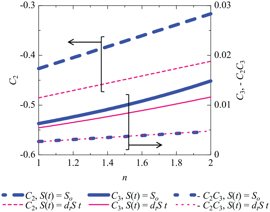
The constants $C_2$ and $C_3$ in the derived solutions include the decay exponent n, as shown in equations (16) and (17). Here, n is the decay exponent of the turbulent kinetic energy in the decaying homogeneous turbulence not affected by the small strain. The value of the decay exponent is slightly larger than unity and depends on the turbulent Reynolds number based on the Taylor scale.^16,22,42 Thus, the derived solutions given by the present study may depend on the turbulent Reynolds number. For a sufficiently high Reynolds number, the decay exponent can be constant and may not depend on the turbulent Reynolds number. In contrast, for a low Reynolds number, the value of the decay exponent can be increased as the turbulent Reynolds number decreases. The dependency of the constants, $C_2$ , $C_3$ , and $C_2{C}_3$ , on the decay exponent n given in equations (16)–(18) is shown in Figure 6, where $C_1$ does not depend on the decay exponent, as shown in equations (16) and (17). As shown in the figure, the absolute value of $C_2$ is decreased as the decay exponent increases. Thus, the effects of $C_2$ , which are shown in Figure 5, may be reduced in the lower-Reynolds-number homogeneous turbulence. In addition, the absolute value of $C_3$ and $C_2{C}_3$ is increased as the decay exponent increases. Thus, the effects of $C_3$ may be more enhanced in the lower-Reynolds-number homogeneous turbulence.

Figure 6.

Dependency of the $C_2$ , $C_3$ , and $-C_2{C}_3$ on the decay exponent n shown in equations (16)–(18). Here, $C_2$ and $C_3$ for the constant variation of $S(t)$ are larger than those for the linear variation, except for the value of $-C_2{C}_3$ . Note that the values of $C_2$ , $C_3$ , and $-C_2{C}_3$ are increased as n increases. The value of n can be increased as the Reynolds number decreases in the decaying grid-generated turbulence. Thus, the value of these coefficients is larger at a lower Reynolds number.

The value of the decay exponent varies significantly among previous studies.^21,22 We investigated the decay exponent value of decaying grid-generated turbulence, as described in the previous work. ¹⁷ The standard $k-ϵ$ model is used to investigate the robustness of decaying homogeneous turbulence in our study. The decay exponent is included as one parameter in the derived governing equations of the standard $k-ϵ$ model, as shown in equation (5). We derive quasi-analytical solutions of the standard $k-ϵ$ model. This analytical solution includes the decay exponent itself and constants, including the decay exponent. For example, the dependence of the constants on the decay exponent is shown in Figure 6. The robustness of decaying homogeneous turbulence is obtained as a quasi-analytical solution, rather than numerical results. The obtained quasi-analytical solutions can represent the effect of the difference in the decay exponent of the decaying homogeneous turbulence.

One equation modeling and effects of second-order terms

The present study next discusses the results from the perspective of one-/two-equation modeling. Here, in the one-equation model, the effects of the small strain on the turbulent kinetic energy could be described using only the governing equation of $f(t)$ . When the magnitude of the small strain is sufficiently small, the small strain only slightly affects the time scale, which is defined as $k(t)/ϵ(t)$ . ³⁵ In this case, since the magnitude of $h(t)$ can be negligibly small, the governing equation of $f(t)$ can be greatly simplified. The analytical solution of the simplified equation of $f(t)$ is derived as $f(t)=\exp (P_o\sigma (t))$ , ³⁵ which does not include $C_3$ or $C_1$ and $C_2$ . Therefore, the effects of the constants, $C_1$ , $C_2$ , and $C_3$ , which are examined in the present study, cannot be found in the results obtained by the one-equation modeling. As shown in Figure 5, the values of $f(t)$ given by the one-equation modeling are significantly smaller than the numerical results for $f(t)$ . For the results for $f(t)$ , the deviation of the derived solutions from that due to the one-equation modeling could be equivalent to the contribution of the two-equation modeling. The derived solutions of $f(t)$ (equation (13)) consist of the first term, which is equal to $f(t)=\exp (P_o\sigma (t))$ , and the other terms described by introducing the two-equation modeling.

A previous study by Suzuki et al. ³⁵ examined the effects of the small strain on the decaying homogeneous turbulence using the governing equations, which are the same as those of the present study (equation (5)). In this previous study, the approximation of $h(t)$ uses two constants, which are equivalent to $C_1$ and $C_2$ in the present study. This previous study enhanced the applicable limit of the derived solutions of $f(t)$ using $C_2$ , as well as $C_1$ . In the present study, the three constants are used to form the approximation of $h(t)$ . As shown in Figure 5, the derived solutions of $f(t)$ for $f(t)\ge 0.01$ could be derived using the third constant $C_3$ . Thus, the present study could clarify the significance of the previously derived solutions using $C_1$ and $C_2$ using $C_3$ , as well as $C_1$ and $C_2$ , for the approximation of $h(t)$ .

The present study examines the effects of the small strain, which is constant or varies linearly. A previous study by Suzuki et al. ³⁶ also discussed the effects of these variations of the small strain on the turbulent kinetic energy and its dissipation using governing equations, which are the same as those of the present study. The previous study used one constant to form an approximation of $h(t)$ , where the constant is equivalent to $C_1$ in the present study. On the other hand, the present study uses the three constants to describe the effects of the constant and linear variations of the small strain. Thus, the derived solutions of the present study are significantly more accurate than those of the previous study. For instance, as shown in Figure 5, the present derived solutions could hold in the region of $0\le \sigma (t)\le 12$ , whereas those of the previous study hold only in the range of $0\le \sigma (t)\le 0.2$ . In addition, the form of $C_1$ in the present study is equal to that derived in the previous study. Therefore, the progress of the present study regarding the effects of the constant and linear variations of the small strain from the previous study was not small.

Conclusion

The present study has obtained the quasi-analytical solution of the turbulence-model equation by focusing on the effects of the small mean strain on the decaying homogeneous turbulence. Here, the small mean strain only slightly affects the anisotropy of the decaying homogeneous turbulence or grid-generated turbulence because a previous experiment on grid-generated turbulence ¹⁶ reported this insensitivity of the anisotropy. Using both the governing equations of the standard $k-ϵ$ modeling and the decay laws of the turbulent kinetic energy k and its dissipation $ϵ$ , refined governing equations for influence functions of the small strain on the turbulent kinetic energy and its dissipation could be derived. The present study derived quasi-analytical solutions of the refined governing equations by solving the equations numerically. The computational conditions of the present numerical simulation are set based on previous experiments on grid-generated turbulence.^1–3 These quasi-analytical solutions describe the relative effects of the small strain on the turbulent kinetic energy and its dissipation in the turbulence mathematically.

In order to derive these quasi-analytical solutions, we focus on the form $h(t)=(f(t)-g(t))/t$ (equation (7)), which is included in the governing equations (equation (5)). Initially, the temporal profile of the form $h(t)$ is numerically examined using the total strain $\sigma (t)$ (equation (8)). Then, the form $h(t)$ could be approximated by a simple function based on the exponential function with three constants, $C_1$ , $C_2$ , and $C_3$ . Here, the approximation of $h(t)$ is refined in order to simplify the derived solutions of the governing equations (equation (12)). Using the refined approximation of $h(t)$ , the derived solutions with the three constants could be given by the governing equations. In addition, the three constants could be formed using the governing equations (equation (16). The forms of the three constants and the derived solutions, that is, quasi-analytical solutions, are validated using the present numerical results. Then, the present study discusses the quasi-analytical solutions from the perspective of the three constants and previous studies. In addition, the dependency of the values of the three constants on the turbulent Reynolds number is discussed. In one-equation modeling, the dependency of the effects on the difference in the variations of the small strain, which is described by the three constants, could not be found.

The quasi-analytical solutions derived in the present study could contribute to the verification, as well as the improvement, of the turbulence modeling used in computational fluid dynamics (CFD) software because the simple mathematical solutions could describe the effects of the small strain in the quasi-analytical solutions of the present study. In the future, a quasi-analytical solution that describes effects of the small strain on other turbulences, for example, forced homogeneous turbulence, should be derived because these turbulence models are also used to simulate forced turbulence as well as decaying turbulence.