Experimental investigation on wake flow structures of Motor Industry Research Association square-back model

Abstract

Since the oil crisis of the last century, drag reduction for vehicles has become the focus of researchers. Currently the world’s major car brands have to seize the sport utility vehicle market. However, the sport utility vehicle models usually have a larger frontal area which brings challenges to drag reduction. This requires a better understanding of flow around sport utility vehicle models. The Motor Industry Research Association square-back vehicle model is similar to the sport utility vehicle geometry and can reflect the typical characteristics of aerodynamics of sport utility vehicle models. In this article, the wake flow structures of a 1/8 Motor Industry Research Association model is measured by particle image velocimetry. The results indicate that there is an obviously “n” type backflow vortex behind the vehicle. In the vertical direction, the vortex rotates from the outside to the inside, meanwhile the vortex rotates from the inside to the outside in the longitudinal direction. There is a velocity deficit region between the vortex and the back of the model which is an important source of drag force. This article summarizes the results of particle image velocimetry measurements from the model tests and obtains a picture of the structures of the wake vortex finally which can provide a theoretical basis for the drag reduction research in the future.

Introduction

Past research shows that the main source of aerodynamics drag is pressure drag, ¹ which is mainly contributed by flow structures in the vehicle wake. ² Researchers paid much attention to the three-dimensional (3D) structures of the car wake because of its obvious engineering significance. Many previous studies about wake structures have been carried out with Ahmed models. Ahmed ³ used a simple 3D bluff body to represent a simplified car body. Based on Ahmed models, Ahmed et al. ⁴ studied the influence of different rear slant inclination angle on the drag coefficient. They found that the drag coefficient peaks when rear slant inclination angle is 30° for Ahmed models. Researchers have done a lot of productive work around the Ahmed models which includes experimental studies^5,6 and numerical studies.^7,8

In order to better understand the structure of the flow field, Motor Industry Research Association (MIRA) model was born in 1980s when European and North American Wind Tunnel operators began a series of correlation research.^9–12 The initial MIRA model was based on mass production vehicle models. Later, Carr ¹¹ at MIRA designed the MIRA Reference Car which is derived from the proportions of “family sized” cars of the era. The design included interchangeable back-ends, that is, as a notchback, fastback, or square back, which have the distinctly different wake structures from each other as identified by Hucho. ¹³ These three back-ends have been the most frequently used, because they represent the most common passenger automobile shapes, and MIRA square-back model is closer to the real sport utility vehicle geometrically compared to Ahmed model.

In early research, Hucho and Sovran ¹⁴ briefly analyzed the wake field of the square-back model, including its effect on aerodynamics drag. Furthermore, there were more studies about the square-back MIRA models which not only focus on the flow analysis of the tail flow field, but also want to improve the tail flow further to achieve drag reduction. Grandemange et al. ¹⁵ studied the effect of the angle of small flaps (or spoilers) located at the top and the bottom of the square-back model trailing edge, and an optimized geometry is found presenting a 5.8% drag reduction compared to the baseline model. Later, PM Palaskar ¹⁶ analyzed the combined effects of different tail taper angles and diffuser on vehicle drag, and suggested that the optimal state of the tail taper angle is 10° and simply increase the diffuser will increase the resistance coefficient of the square-back model. Littlewood and colleagues^17–19 conducted a series of studies around the square-back model, including passive and active optimization. They investigated the effect of different roof trailing edge on aerodynamic drag. The results ¹⁷ showed that C_d can be reduced by 4.4% (13 counts) when the chamfer angle is 12°. The study of Littlewood and Passmore ¹⁹ reported drag reductions of up to 8 counts and lift reductions of up to 32 counts by introducing slats on the back. They also studied the effect of active flow control technology on square-back model. However, it is found that C_d increased for most steady blowing cases which reminds that researchers need a better understanding of wake structure to use active flow control technology properly. In addition, Bearman and colleagues^20,21 used particle image velocimetry (PIV) technique to measure a 1/8 scale vehicle, and they found obvious difference between time-averaged velocity field and instantaneous velocity field of the wake.

Many previous researchers have analyzed the effect of the change in the tail structure on the flow field structure. However, few studies make systematic detailed description of the tail flow field structure and analysis of the mechanism for the tail vortex of the original MIRA square-back model. The objective of this study is to visualize the wake flow structures around an MIRA square-back model using PIV technique to provide a theoretical basis for the drag reduction research in the future. In this article, the experimental setup will first be described. Next, results of time-averaged velocity field, turbulence intensity, and velocity deficit of the wake are presented and discussed. Finally, some conclusions will be drawn.

Experimental setup

Wind tunnel facility and vehicle model

PIV experiments were conducted in an automotive wind tunnel at Jilin University. It is an 8-m long, 4-m wide, and 2.2-m high open circuit wind tunnel. The maximum velocity of the tunnel is approximately 60 m/s, and the nozzle area is 8.4 m². The detailed geometric dimensions of the original MIRA square-back model are shown in Figure 1(a), which is 4165 mm in length, 1625 mm in width, and 1421 m in height. However, the objective of this research is investigating wake structures as mentioned above. It is difficult to measure flow structures of a full-size model using PIV. Meanwhile, considering experimental conditions, 1/8 MIRA square-back model is the final choice. The 1/8 MIRA square-back test model is shown in Figure 2, which is 520 mm in length, 203 mm in width, and 177 m in height. Due to the size of the experimental model, the boundary layer may have a significant effect on the flow structures around the model. In order to avoid this, a test bench was designed with a thin plate with a curved leading edge, which was located in the middle of wind tunnel outlet as shown in Figure 2. This design was introduced by Narasimha and Prasad ²² to avoid flow separation. The square-back model is placed at the distance from the front edge of the plate to 350 mm, and is located at the center of the left and right symmetry.

Figure 1.

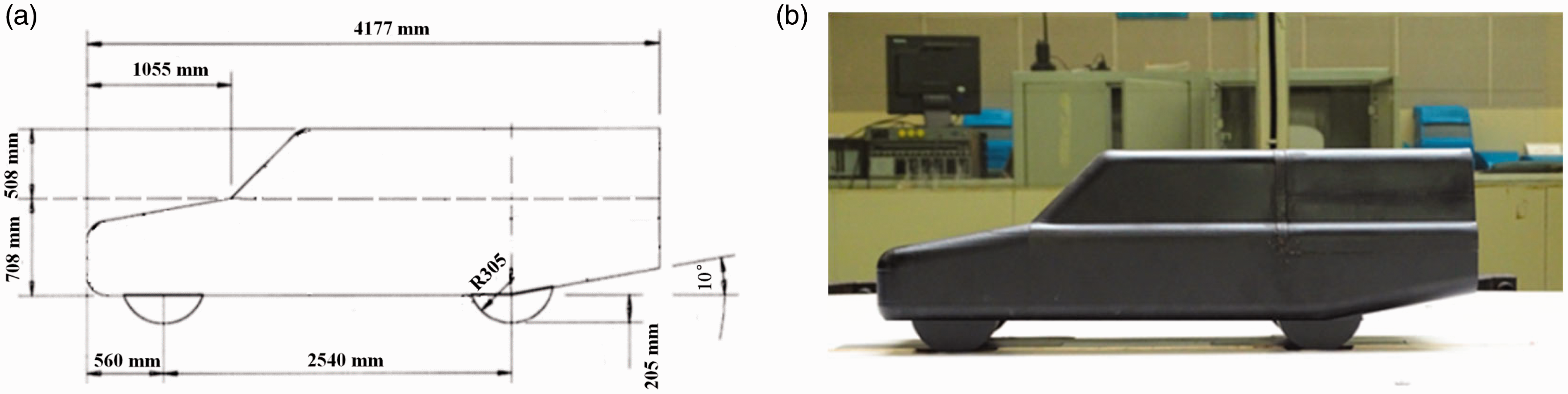
Detailed geometric figure of square-back model: (a) original size of MIRA square-back mode and (b) 1/8 scale test mode in wind tunnel.

Figure 2.

Setup of PIV measurements. (a) for longitudianl planes, (b)for transverse planes, (c) for spanwise planes.

Measurements were conducted at the free stream velocity which is 27.78 m/s, corresponding to a Reynolds number, Re = 9.18 × 10⁵. The non-uniformity of free stream in the test section was 0.1%. The streamwise turbulence intensity was about 0.5% in the absence of the test model for the test case velocity. The blockage ratio of the frontal surface of the model to the rectangular wind tunnel outlet was 4.1% which means that the blockage effect of this model can be neglected as long as the blockage ratio is under 5% according to Farell et al. ²³

PIV measurements

The schematic of experimental setup is shown in Figure 2. A TSI PIV system was used to measure flow field around the model. The flow field was illuminated using two Nd-YAG lasers, each with a maximum energy output of 200 mJ/pulse. The output beams are shaped into a 1∼2-mm thick laser sheet normal to the free stream by a cylindrical lens. The lasers were synchronized to illuminate the flow twice with a short time delay between the two exposures. The working frequency is 10 Hz, and the pulse interval can be adjusted from 200 ns to 0.1 s. The test wind velocity is 27.78 m/s, and the time interval of setting PIV pulse is 15 microsecond. The tracer particles used in this experiment are smoke, heated by vaporization of smoke oil via smoke generator. The particle size of smoke particles is 10 μm. The light scattered by the seeding particles was recorded with a charge-coupled device (CCD) camera. The field of view of PIV images was 350 × 300 mm. The number of images needs to be adequate for determining both mean and fluctuating flow fields, ²⁴ so a total of 1200 PIV images were recorded at each plane.

The coordinate system (Figure 2) follows the right-hand rule and is defined such that x, y, and z are directed along the longitudinal flow, spanwise, and vertical (transverse) directions, respectively. In order to capture accurately the 3D flow structures, PIV measurements were performed in a number of planes, including y = 0 mm (symmetry plane), 50 mm plane, z = –60 mm, –34 mm, –15 mm, 32 mm plane, and x = 50 mm, 120 mm plane. Different measurement planes are illustrated in Figure 3. For the measurements in the y–z plane, a camera was vertically placed in the tunnel where x = 2000 mm, equivalent to four model lengths. At such a distance downstream of the PIV imaging plane, the camera has a negligibly effect on the measurement. The PIV data are processed by Insight software that comes from TSI.

Figure 3.

Different planes locations in three orthogonal planes.

Analysis of longitudinal planes

As mentioned above, the aerodynamics drag of the vehicle is mainly contributed by the flow separation of the wake flow. A better understanding of the wake structure can help vehicle designers find out which areas have obvious flow separation and momentum exchange, and then researchers can apply drag reduction measures to these areas such as active flow control. The flow field structures of wake can also indicate where the low-velocity zone causing drag is and how the low-velocity zone recovered. However, since the wake structure is a complex 3D structure, it is difficult to describe its structure from a single-direction plane. Therefore, three parts are used to describe the flow field structure of different direction sections in this article. In this part, the experiment results of longitudinal planes will be showed and discussed first.

Four kinds of images will be discussed, including the contours of dimensionless velocity magnitude with streamline and vector, the contours of time-averaged vorticity, and the contours of time-averaged turbulence intensity. With the help of contours of dimensionless velocity magnitude with streamline and vector, we can observe large flow structure and stable vortex at this plane. Next, the contours of time-averaged vorticity will be showed. Vorticity characterizes shear and rotation of fluid micelles which can provide another view of the flow field. Finally, the results of time-averaged turbulence intensity will be presented to show which area of the flow field has high-level velocity pulsation which means that there is a large number of transient small vortices and intense momentum exchange in this area.

Time-averaged velocity field

Because of the special tail structure of the square-back model, data of two longitudinal cross planes (x = 50 mm and x = 120 mm) were selected for analysis. It should be noted that the results shown below are the components of the 3D physical quantity on the plane. For example, the velocity magnitude of this plane can be considered as the component of the 3D velocity magnitude but not including the velocity in the x direction. It mainly characterizes the lateral flow of wake.

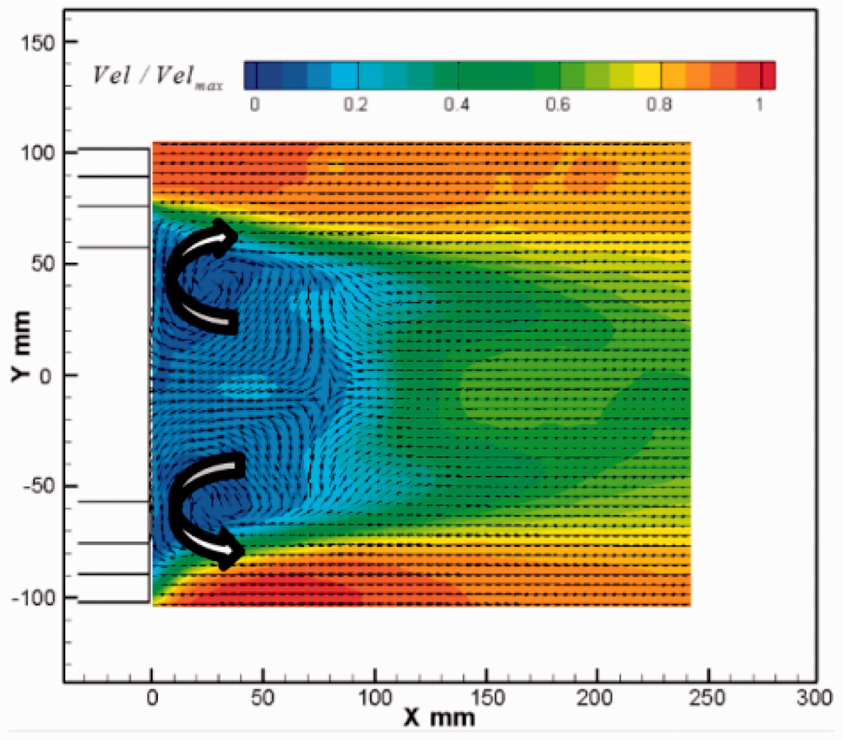
The contours of time-averaged dimensionless velocity magnitude with streamline and vector at the longitudinal plane of x = 50 mm are shown in Figures 4 and 5, respectively. At the plane of x = 50 mm, the velocity magnitude below the vehicle is larger than the velocity magnitude above the vehicle body which means that the lateral flow under the vehicle is more intense than the lateral flow in the upper part. It is because that the section is very close to the rear of the car, and the disturbance of the wheel causes a wake with large lateral velocity below the vehicle. Meanwhile, the streamline indicates that some small vortices exist in the area near the outline of the vehicle in Figure 4. The contours with vector also show this point in Figure 5. We can also find that the vortex on the right side rotates clockwise but the vortex on the left side rotates anticlockwise in Figure 5. It is because that the vehicle geometry is symmetrical about the middle section (y = 0), the vortex system produced is also symmetrical about the middle section roughly.

Figure 4.

The contour of time-averaged dimensionless velocity magnitude with streamline at the longitudinal plane of x = 50 mm.

Figure 5.

The contour of time-averaged dimensionless velocity magnitude with vector at the longitudinal plane of x = 50 mm.

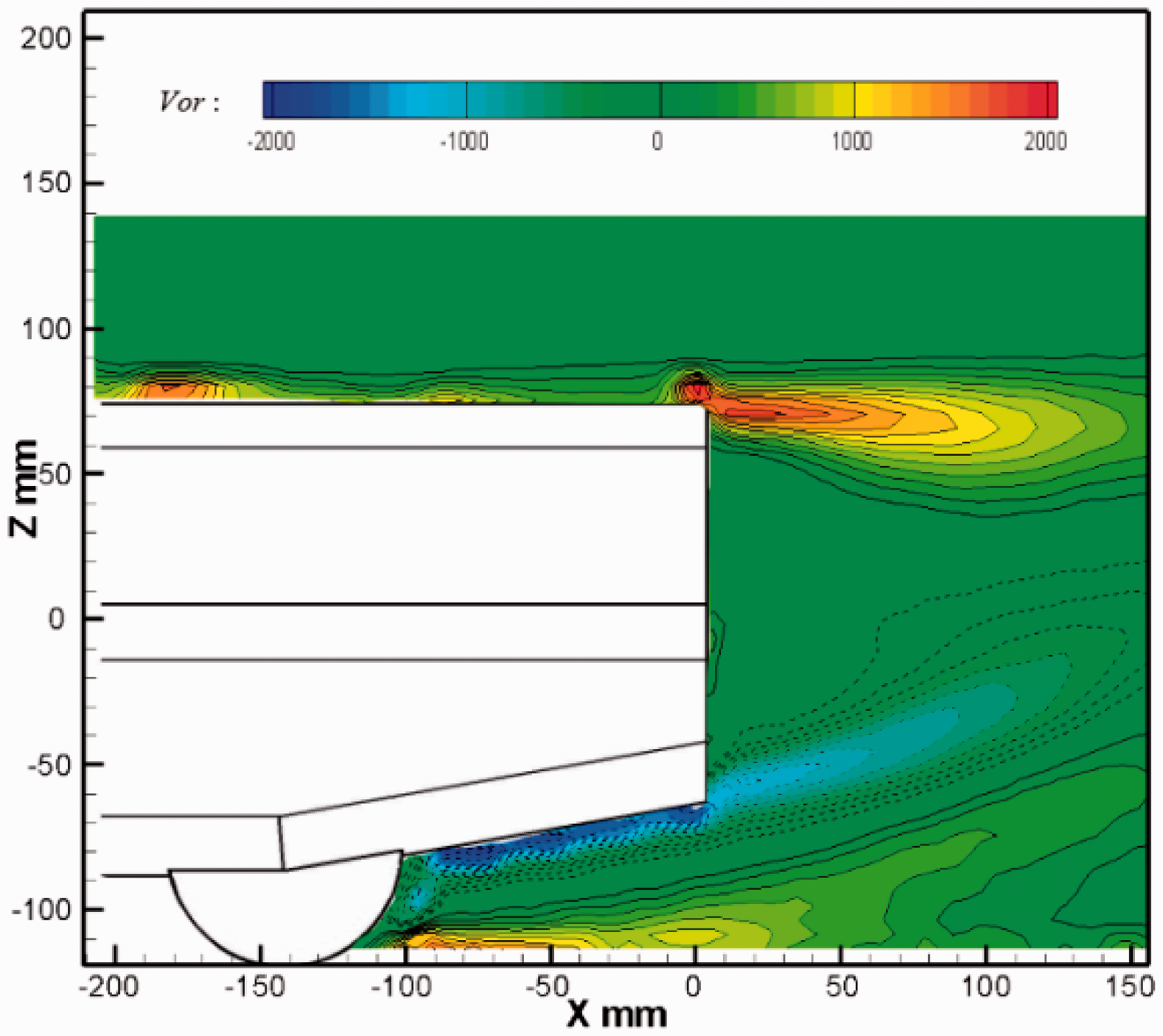
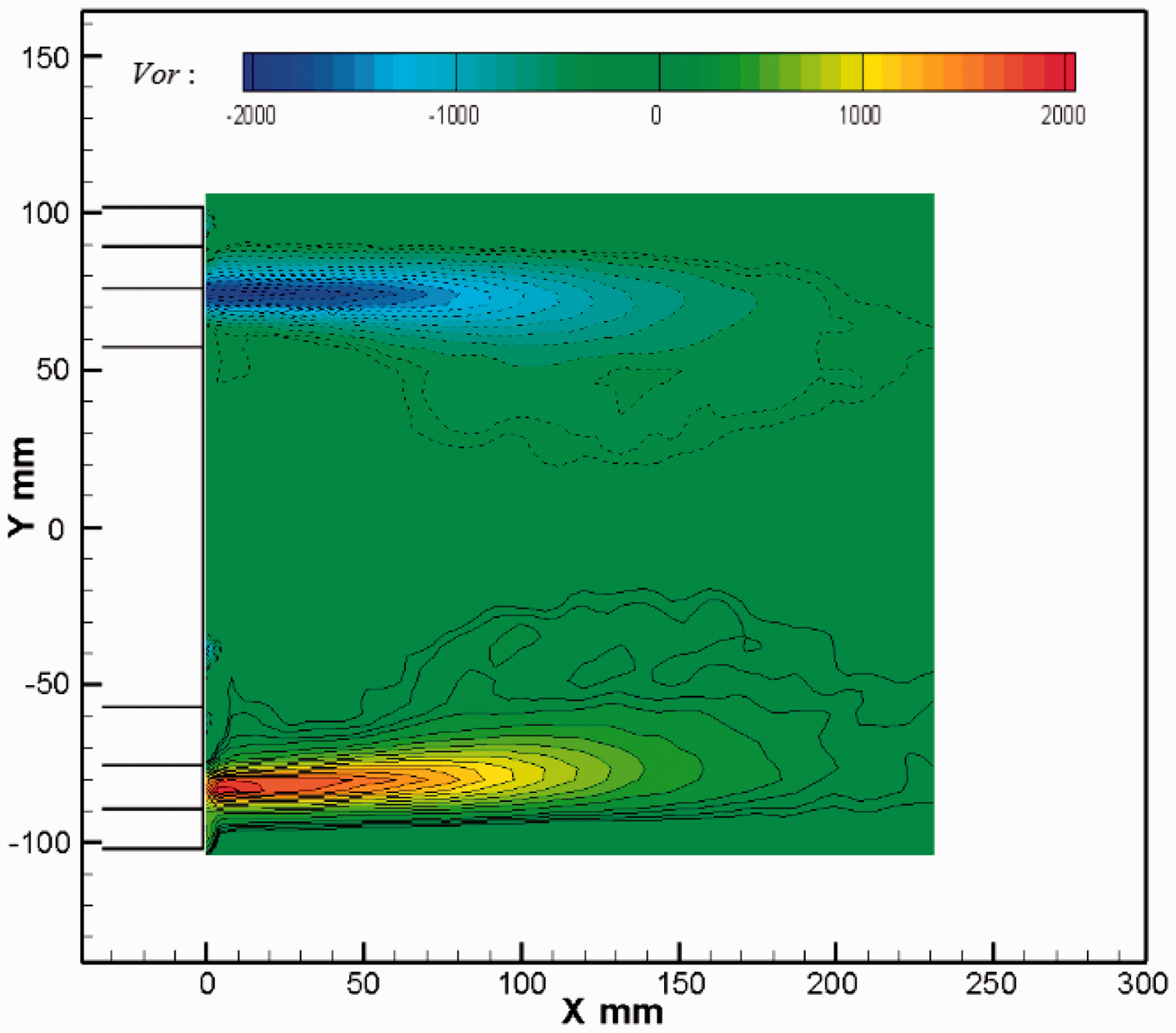
Figure 6 provides more details of the flow field by the contour of time-averaged vorticity at the longitudinal plane of x = 50 mm. The positive and negative values of the vorticity indicate the direction of rotation. Positive values which color is close to blue indicate anticlockwise rotation, and negative values which color is close to yellow indicate clockwise rotation. We can draw conclusions about the symmetry of the flow field consistent with the above. It can be also found from Figure 6 that there is a pair of small vortices on both sides of the tail, which may be generated by the air flow passing through the roof. The shear layer along the two sides is separated at the tail to form side vortices marked by A vortex. There is an alternate vortex at the lower trailing edge, which is named C vortex. We can see that there is a vortex on both sides of the bottom of the tail, which is named D vortex, which is formed by the interaction between the upward air flow at the upturned angle and the airflow on both sides of the vehicle tail. In the gap between the bottom of the car body and the ground, a pair of vortices is generated near the ground named B vortex. In summary, the main vortex structure at the plane of x = 50 mm generated by the rear end of a square-back car is summarized in Figure 6.

Figure 6.

The contour of time-averaged vorticity at the longitudinal plane of x = 50 mm.

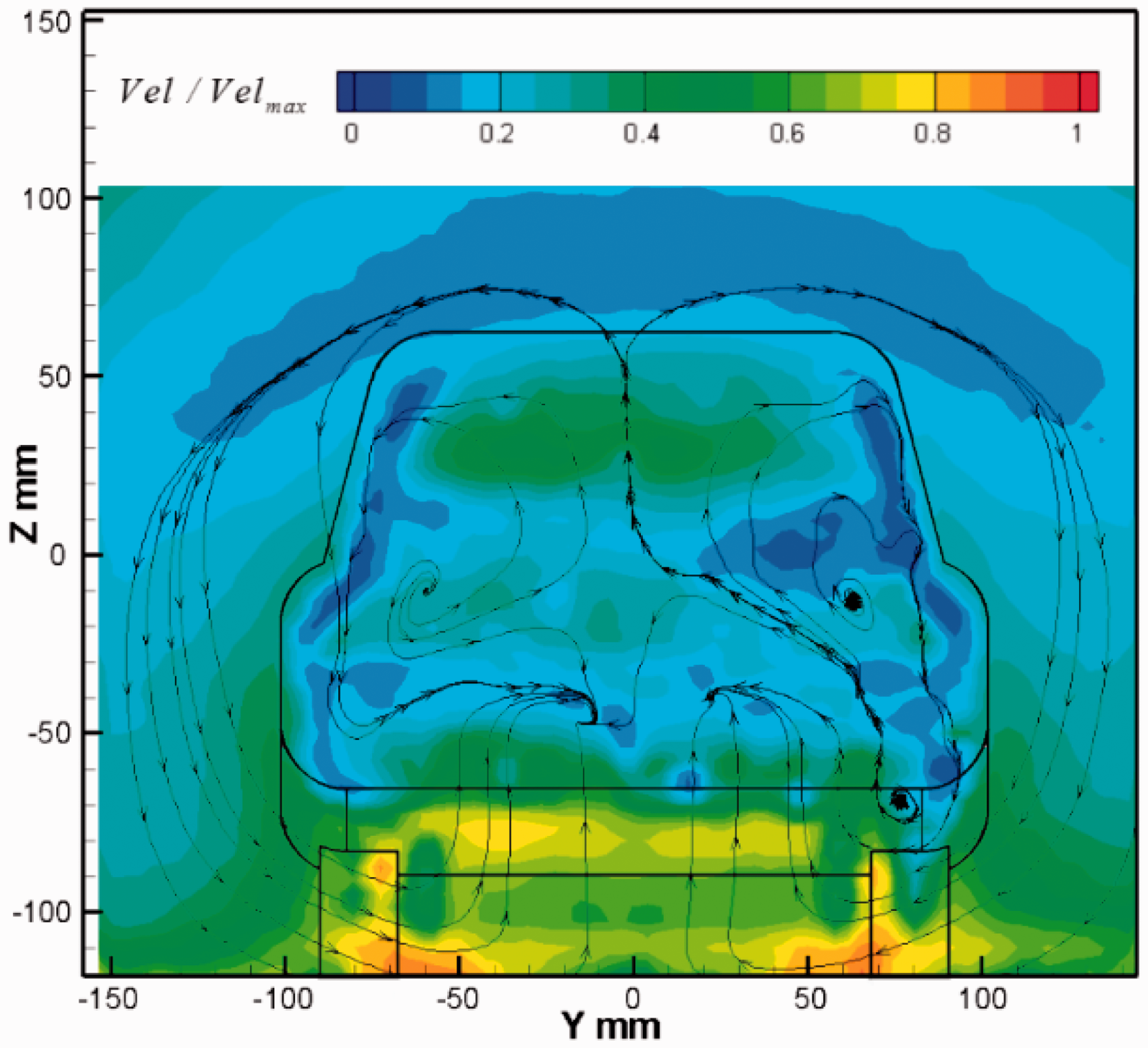
The contour of time-averaged dimensionless velocity magnitude with streamline at the longitudinal plane of x = 120 mm is shown in Figure 7. It can be found from the contour of dimensionless velocity magnitude that the main lateral flow occurs in the central region of the wake. The image of the streamline shows a large backflow in the central region of the wake in Figure 7 at the plane of x = 120 mm. Figure 8 shows the contour of time-averaged dimensionless velocity magnitude with vector which shows the flow field structure further. It can be seen that the large flow field structure in the backflow zone is two pairs of symmetrical vortices. There is also a pair of vortices near the ground which can be seen as extension of B vortex.

Figure 7.

The contour of time-averaged dimensionless velocity magnitude with streamline at the longitudinal plane of x = 120 mm.

Figure 8.

The contour of time-averaged dimensionless velocity magnitude with vector at the longitudinal plane of x = 120 mm.

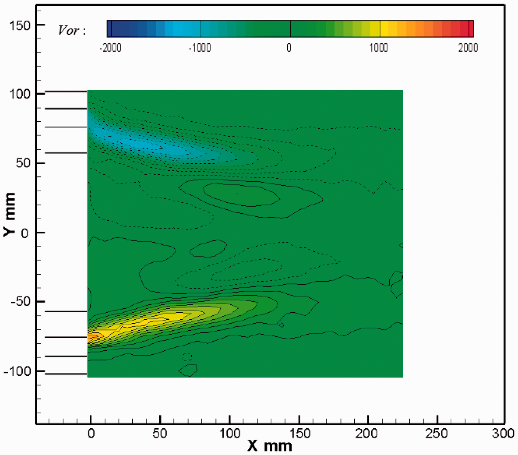
As shown in Figure 9, the flow structures of wake become clearer with the development of vortex. The contour of time-averaged vorticity shows that the vortices are gradually joined together and form an “n” shape to surround the tail. The “n” shaped vortex is a backflow vortex to the interior of the rear which is an important feature of the wake vortex structure. Meanwhile, we can also observe significant vorticity near the ground which represent the extension of B vortex.

Figure 9.

The contour of time-averaged vorticity at the longitudinal plane of x = 120 mm.

Analysis of turbulence intensity

Some large and stable flow field structures at the longitudinal planes have been discussed above. However, the information of transient and small flow structures may be missed in the time-averaged results. In order to investigate the disorder and turbulence of the flow field, turbulence intensity based on statistical results of 1200 PIV images is introduced. Turbulence intensity is defined by the ratio of standard deviation of wind velocity to average wind. Areas with high turbulence intensity usually mean more disordered small vortices which bring more momentum exchange.

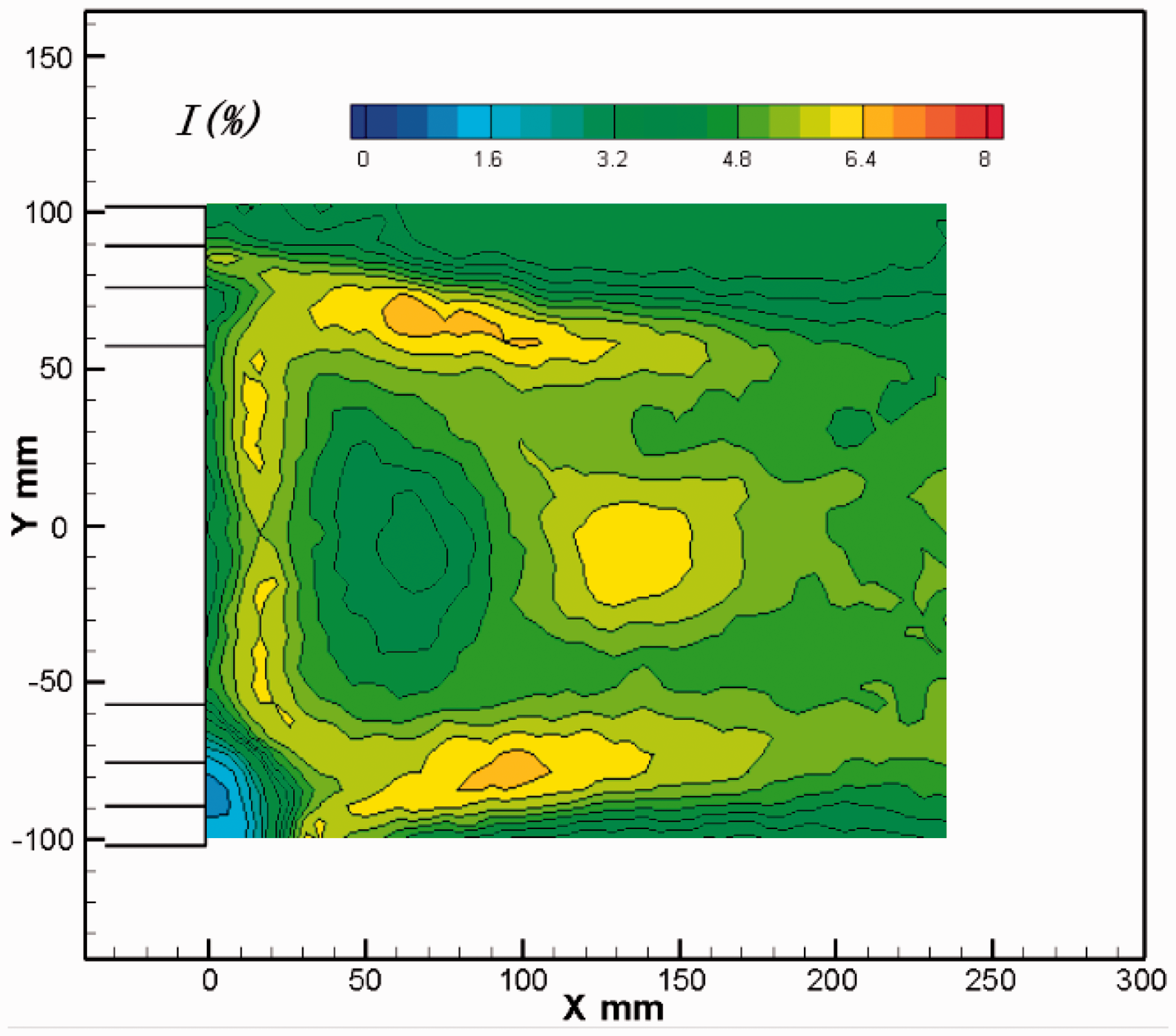
The contour of turbulence intensity at the longitudinal plane of x = 50 mm is showed in Figure 10. As we can see, a high-turbulence area is near the roof and a high-turbulence area is near the ground. Considering with the plane is close to the body, it is possible that the separation of the flow around the roof and the wheel causes the local high turbulence intensity.

Figure 10.

The contour of turbulence intensity at the longitudinal plane of x = 50 mm.

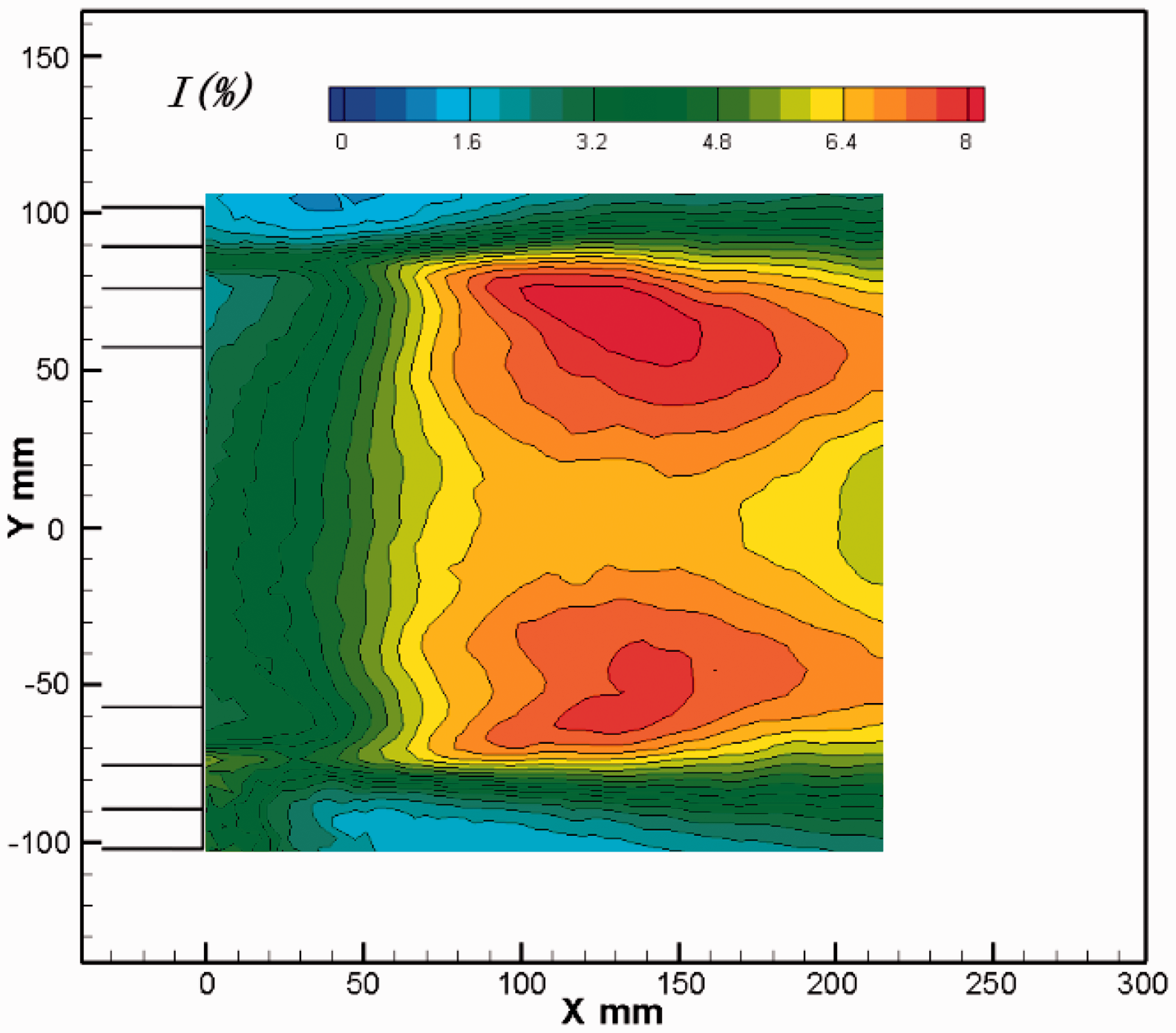
Figure 11 shows the contour of turbulence intensity at the longitudinal plane of x = 120 mm. It can be clearly seen that the high turbulence intensity region corresponds to the high-vorticity region in Figure 9 roughly. Due to the n-type vortex system, there is also an n-type high turbulence intensity region on this plane. Meanwhile, the area of the n-type high-turbulence area is larger than the n-type high turbulence intensity region. It is because in the development of the wake, there is a process of breaking the large vortex into small vortices, which will increase the local turbulence and momentum exchange. The increase in turbulence intensity can promote the mix of the core region of the wake with the mainstream which is also found in the analysis of the spanwise planes below.

Figure 11.

The contour of turbulence intensity at the longitudinal plane of x = 120 mm.

Analysis of spanwise planes

PIV results of two spanwise planes (y = 0 mm and y = 50 mm) are presented in this part. The contours of time-averaged velocity field and turbulence intensity are discussed to show the structures of wake. Furthermore, due to the velocity deficit in the direction of x contributes a lot to the drag, the velocity deficit of the wake at different position in the direction of x was calculated and presented in this part.

Time-averaged velocity field

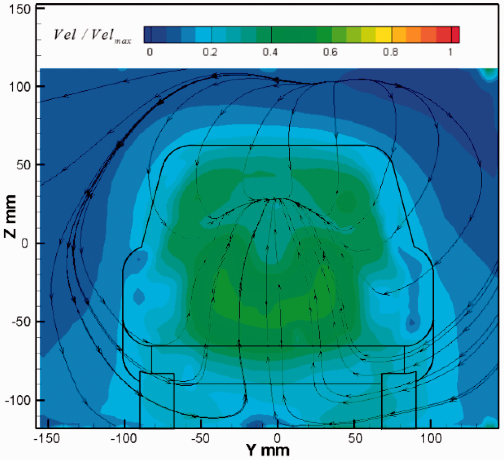
Figure 12 shows the contour of time-averaged dimensionless velocity magnitude with streamline at the spanwise plane of y = 0 mm. It can be seen that there is a large low-velocity zone at the rear of the vehicle. The two sides of the low-velocity zone are relatively high-velocity airflow from the roof and the underbody. As the flow of airflow, the width of the low-velocity region gradually decreases in the x direction.

Figure 12.

The contour of time-averaged dimensionless velocity magnitude with streamline at the spanwise plane of y = 0 mm.

wIt can be seen from the streamline in Figure 12 that there are two obvious vortices behind the rear of the MIRA model which are positioned at the interface between the wake and the free flow. This may be caused by the large velocity difference between the low-velocity region of the wake and the airflow at the upper and lower sides of the vehicle body. There is a strong shear and rotation effect at the interface between the wake and the free flow, which promotes the formation of these two vortices. At the same time, it can also be observed in Figure 13 that there is a phenomenon that high-velocity fluids on both sides flow into the core of wake. Along with this flow pattern, the low-velocity region of the wake is gradually narrowed. Figure 14 shows the contour of time-averaged vorticity at the same plane of y = 0 mm. There are three obvious high-vorticity areas, two of which correspond to the vortex positions showed in Figures 12 and 13. It is worth noted that there is also a high-vorticity area near the ground. It is due to the development of the ground boundary layer where there is strong shearing effect.

Figure 13.

The contour of time-averaged dimensionless velocity magnitude with vector at the spanwise plane of y = 0 mm.

Figure 14.

The contour of time-averaged vorticity at the spanwise plane of y = 0 mm.

The contours of time-averaged dimensionless velocity magnitude with streamline and vector at the spanwise plane of y = 50 mm are shown in Figures 15 and 16, respectively. This plane is closer to the wheel in the y direction. As we can see, the characteristics of time-averaged flow field at plane of y = 50 mm is similar to the plane of y = 0 mm. There are also two obvious vortexes behind the rear of the MIRA model. However, the position of vortexes is more near the rear end of the model in Figure 15. It can be found that obvious reflow flow is also approaching the rear of the car in Figure 16. At the same time, the area of the high-velocity airflow area under the car body is reduced because of blocking effect of the wheel on the flow below.

Figure 15.

The contour of time-averaged dimensionless velocity magnitude with streamline at the spanwise of y = 50 mm.

Figure 16.

The contour of time-averaged dimensionless velocity magnitude with vector at the spanwise plane of y = 50 mm.

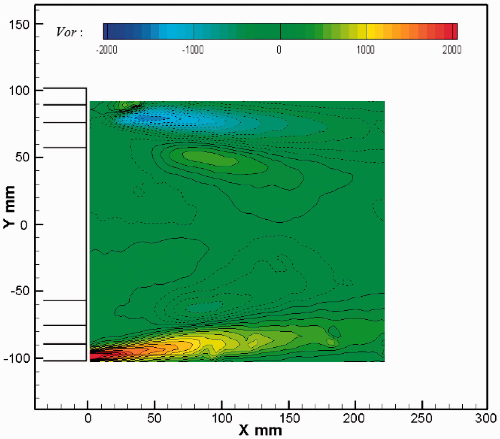
Figure 17 shows the contour of time-averaged vorticity at the spanwise plane of y = 50 mm, it is basically similar to the result of plane of y = 0 mm in Figure 14. Due to the presence of the reflow vortexes, there are two high-vorticity areas near the upper and lower sides of the vehicle body. However, the high-vorticity area near the ground is shorter than the same area in Figure 14. It is because that the blocking effect of the wheel on the flow below, resulting in a decrease in the vorticity in this area.

Figure 17.

The contour of time-averaged vorticity at the spanwise plane of y = 50 mm.

Analysis of turbulence intensity

The contour of turbulence intensity at the spanwise plane of y = 0 mm is showed in Figure 18. As it shown, the turbulence intensity is lowest in the area close to the rear of the car, and the turbulence intensity gradually increases along the x direction. Compared to Figures 12 and 13, it can be seen that the location of the high turbulence intensity region is at the interface of the low-velocity wake and free flow. It is pointed that large and stable vortices in Figure 12 may not have much contribution to momentum exchange. We can speculate that the large number of transient small vortices formed by the broken large vortex complete the main task of momentum transfer, thus helping the free flow and the wake to mix with each other. These areas where high levels of momentum exchange occur are the areas of high turbulence intensity in Figure 18. The contour of turbulence intensity at the spanwise plane of y = 50 mm is showed in Figure 19, the distribution of turbulence intensity is very similar to that in Figure 18. The difference is that there is a row of high turbulence intensity area on the roof. The possible reason is that the section of y = 50 mm is very close to the outside of the model which can be seen in Figure 3. The high-turbulence area here may correspond to the vortex at the top edge of the car.

Figure 18.

The contour of turbulence intensity at the spanwise plane of y = 0 mm.

Figure 19.

The contour of turbulence intensity at the spanwise plane of y = 50 mm.

Analysis of velocity deficit of the wake

The momentum deficit of the wake in the direction of drag which is the direction of x in this article is seen as an important indicator of drag. Considering the small Mach number of the flow in this experiment, the density does not change much, so the velocity deficit $U/U_{\infty }$ is used to measure the degree of momentum deficit of the wake in this part.

$U/U_{\infty }$ represents the degree of velocity deficit of wake in the x direction. If the value of $U/U_{\infty }$ is closer to 0, the velocity deficit is more serious. Figures 20 and 21 show the time-averaged contour of $U/U_{\infty }$ at the spanwise plane of y = 0 mm and y = 50 mm, respectively. As we can see, the red color area in the figure represents the free-flow area. The fluid in this area is less affected by the car body, so the velocity deficit is also less in this area. The blue color area in the figure represents the core low-velocity zone of the wake where the velocity deficit is very serious. It can be found that there is an area where $U/U_{\infty }$ is less than 0 in dark blue color area which means that there is a reflow in this area. Green area between the low-velocity zone and free flow represents velocity recovery zone. In this area, the airflow velocity gradually recovers to the same level with free flow. It is worth pointing out that velocity recovery area in Figures 20 and 21 happens to be the high-level turbulence intensity area in Figures 18 and 19 which reaches agreement with the conclusion that the transient small vortex contributes to momentum transport. Comparing Figure 20 with Figure 21, the core low-velocity zone of the wake at the spanwise plane of y = 50 mm is smaller which means that the velocity deficit of the center section (y = 0 mm) of the car is more serious than the edge section (y = 50 mm). To further discuss the velocity deficit of wake in detail, six feature lines separated by 30 mm from each other were chosen to present the variation of velocity deficit at different locations. The schematic diagram of different locations of feature lines is shown in Figure 22.

Figure 20.

The time-averaged contour of $U/U_{\infty }$ at the spanwise plane of y = 0 mm.

Figure 21.

The time-averaged contour of $U/U_{\infty }$ at the spanwise plane of y = 50 mm.

Figure 22.

Schematic diagram of different locations of feature lines.

Figure 23 shows the variation of velocity deficit in the wake at different positions at the plane of y = 0 mm. The part of the curve whose value of $U/U_{\infty }$ is less than 1 can be regarded as the velocity deficit zone. If the value of $U/U_{\infty }$ is less than 0, then the area can be regarded as reflow zone. There are two obvious velocity deficit zones. The higher one is caused by wake, and the lower one near the ground is caused by boundary layer development. As we can see, the velocity deficit zone caused by wake of line at x = 5 mm is the largest. Along the x direction, the velocity deficit zone caused by wake is getting smaller while the velocity deficit zone caused by boundary layer is getting larger. It is because that the breaking of the large vortex into a small vortex contributes to the exchange of momentum between the high- and low-velocity fluids as the wake develops; thus, the area of the velocity deficit zone of wake is reduced. At the same time, the thickness of the boundary layer also increases as the boundary layer develops; thus, the area of the velocity deficit zone of boundary layer is increased. We can also conclude that the main reflow zone is between the x = 5 mm and x = 125 mm, and the strongest reflow occurred at around the x = 65 mm.

Figure 23.

Variation of velocity deficit in the wake at different positions at the spanwise plane of y = 0 mm.

Figure 24 shows the variation of velocity deficit in the wake at different positions at the plane of y = 50 mm. The variation of velocity deficit is similar to that at the plane of y = 0 mm compared with Figure 23. However, the area of velocity deficit zone and reflow zone is both smaller than that at the plane of y = 0 mm. We can also found that the development of the ground boundary layer is limited due to the influence of the wheels, and the area of the velocity deficit area close to the ground is small. The main reflow zone is also between the x = 5 mm and x = 125 mm, and the strongest reflow occurred at around the x = 65 mm.

Figure 24.

Variation of velocity deficit in the wake at different positions at the spanwise plane of y = 50 mm.

Figure 25.

The contour of time-averaged dimensionless velocity magnitude with streamline at the transverse plane of z = 32 mm.

Figure 26.

The contour of time-averaged dimensionless velocity magnitude with vector at the spanwise plane of z = 32 mm.

Analysis of transverse planes

Time-averaged velocity field

The PIV results of flow filed at transverse planes can provide more information about the “n” shaped vortex. The contours of time-averaged velocity field and turbulence intensity of four transverse planes which are z = 32 mm, z = –15 mm, z = –34, and z = –60 are presented in this part.

Figures 25–32 show the contours of time-averaged dimensionless velocity magnitude with streamline and vector the transverse plane of four planes. It can be found that velocity magnitude on both sides of the body is higher than the core area of wake at all the four planes. The shape of the low-velocity region changes as the position of the plane changes. At the plane of z = 32 mm, the shape of the low-velocity region (Vel/Vel_max < 0.15) is convex, and the low-velocity region in the middle is longer than the low-velocity region on both sides. However, the shape of the low-velocity region is like a trapezoid, the low-velocity region in the middle and the low-velocity region on both sides are flush at the plane of z = –15 mm in Figure 27. Furthermore, the shape of the low-velocity region is concave, the low-velocity region in the middle is shorter than the low-velocity region on both sides in Figure 29. At last, the low-velocity region has disappeared, but there is an elliptical relatively high-velocity area at the plane of z = –60 mm in Figure 31. It is the yellow color region which may be influenced by the high-velocity flow under the body in Figure 20. We can also conclude that the velocity difference between the high-velocity flow and the low-velocity flow is gradually decreasing along the negative direction of the z-axis.

Figure 27.

The contour of time-averaged dimensionless velocity magnitude with streamline at the transverse plane of z = –15 mm.

Figure 28.

The contour of time-averaged dimensionless velocity magnitude with vector at the transverse plane of z = –15 mm.

Figure 29.

The contour of time-averaged dimensionless velocity magnitude with streamline at the transverse plane of z = –34 mm.

Figure 30.

The contour of time-averaged dimensionless velocity magnitude with vector at the transverse plane of z = –34 mm.

Figure 31.

The contour of time-averaged dimensionless velocity magnitude with streamline at the transverse plane of z = –60 mm.

Figure 32.

The contour of time-averaged dimensionless velocity magnitude with vector at the transverse plane of z = –60 mm.

As for the flow structures, the main feature on transverse plane is a pair of rotating vortices whose position changes at different planes position. As we can see in Figure 26, this pair of rotating vortices is located at the interface between the low-velocity area and the recovery area. As the plane moves down, it can be seen that this pair of vortices move toward the rear of the car and get closer and closer to each other in Figures 28 and 30, and there is no obvious flow structure in Figure 32 at the plane of z = –60 mm.

Figures 33–36 show the contours of time-averaged vorticity at four different planes which are z = 32 mm, z = –15 mm, z = –34 mm, and z = –60 mm. The high-vorticity areas in these figures are mainly on both sides of the car body where the flow separation phenomenon is obvious after the rear end of the MIRA square-back model. As we can see, the high-vorticity area is basically between the high-velocity zone and the low-velocity zone which is the green area in Figures 25–32. It can be speculated that these vortexes on the transverse planes are shear vortexes formed by the large velocity difference between wake core zone and fluid on both sides. And the intensity of vorticity gradually decreases along the negative direction of the z-axis. For example, the vorticity at transverse plane of z = 32 mm is higher and concentrated on both sides of the car body. However, the vorticity at transverse plane of z = –60 mm is much lower and there are many small vorticity areas besides the both sides. We can conclude that the flow separation and vortexes on the plane near the roof is more intense than the plane near the ground in the wake of MIRA square-back model.

Figure 33.

The contour of time-averaged vorticity at transverse plane of z = 32 mm.

Figure 34.

The contour of time-averaged vorticity at transverse plane of z = –15 mm.

Figure 35.

The contour of time-averaged vorticity at transverse plane of z = –34 mm.

Figure 36.

The contour of time-averaged vorticity at transverse plane of z = –60 mm.

Analysis of turbulence intensity

Figures 37–40 show the contours of time-averaged vorticity at four different planes which are z = 32 mm, z = –15 mm, z = –34 mm, and z = –60 mm. As discussed in the results for longitudinal planes and spanwise planes, it can be found that the region where there is a stable large flow structure exists is not a high turbulence intensity region. Compared with Figures 25–32, we can found that these areas of high turbulence intensity are where the velocity gradient is large. The large shear vortex breaks into a large number of unstable small vortices to form a momentum conveyor belt, which helps the velocity recovery of the wake. We can also found that the turbulence intensity gradually decreases from Figures 37–40 which means that momentum exchange between fluids on the plane near the roof is more intense than that near the ground.

Figure 37.

The contour of turbulence intensity at the transverse planes of z = 32 mm.

Figure 38.

The contour of turbulence intensity at the transverse planes of z = –15 mm.

Figure 39.

The contour of turbulence intensity at the transverse planes of z = –34 mm.

Figure 40.

The contour of turbulence intensity at the transverse planes of z = –60 mm.

Analysis of velocity magnitude from 3D view

To provide a better vision of the flow structures of wake, Figures 41–43 summarize the velocity magnitude of three orthogonal planes, respectively. The contours of time-averaged velocity magnitude without dimensionless of the plane in the same direction are shown under the same legend. The picture is set to be transparent, and the distance between the planes is appropriately increased for better display. As we can see in Figure 41, the lateral flow on plane of x = 120 mm is more intense than plane of x = 60 mm, especially in the area influenced by the wake. It can be said that the velocity deficit in the x direction is recovering but the cross flow in the y direction is stronger with the development of the wake. Next, Figure 42 shows the contours of time-averaged velocity magnitude of spanwise planes from 3D view. It can be found that the flow patterns on planes of y = 0 mm and y = 50 mm are basically the same. It can both be observed that the triangular low-velocity zone is behind the vehicle body which contributes a lot to the drag. However, the velocity of airflow near the ground at the plane of y = 50 mm is lower than the y = 0 mm.

Figure 41.

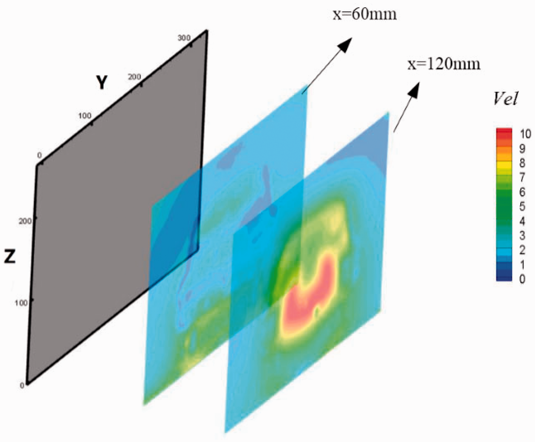
The contours of time-averaged velocity magnitude of longitudinal planes from 3D view.

Figure 42.

The contours of time-averaged velocity magnitude of spanwise planes from 3D view.

Figure 43.

The contours of time-averaged velocity magnitude of transverse planes from 3D view.

Finally, Figure 43 shows the contours of time-averaged velocity magnitude of four different transverse planes from 3D view. We first notice that the area of the low-velocity zone decreases from top plane (z = 32 mm) to bottom plane (z = –60 mm) which confirms the outline of low-velocity zone in Figure 42. Meanwhile, starting from plane A, the speed zone in the middle recovers faster than on both sides at the plane of z = 15 mm and z = –34 mm. An n-type low-velocity zone is formed looking from the top down. Considering the shear effect between the low-velocity airflow and the high-velocity airflow, it is easy to generate a vortex system. It can explain how the n-type vortex is formed in Figures 9 and 11. However, there is a relatively high-velocity zone in the middle of the image of velocity magnitude at the plane of z = –60 mm. It is because of the different velocity in the middle and on both sides in the y direction which can also be found in Figure 42. In short words, plane of z = 32 mm is more affected by the roof airflow, while plane of z = –60 mm is more affected by the flow near the ground. Multiple flow structures at different planes together form the complex n-type vortex.

Conclusion

The wake flow field of MIRA square-back model is investigated in this article using PIV measurement technique. Time-averaged velocity field and turbulence intensity of three orthogonal planes are showed and discussed. The velocity deficit was introduced to discuss the influence of wake flow field structure on drag furthermore. The purpose of this article is to draw a better picture of the wake flow structure of MIRA square-back model. With the help of results of PIV measurement on three orthogonal planes, we found some typical vortexes and flow phenomena. We also observed the shear effect between the wake low-velocity zone and the free flow which may be the main cause of various flow structures in the wake. Last but not the least, we recognize the importance of transient small vortexes on the momentum transfer in the wake of MIRA square-back model by the analysis of turbulence intensity. The structures of the wake vortex can be obtained as shown in Figure 44.

Figure 44.

The structure of the wake vortex of MIRA square-back model.

Based on previous analysis, main conclusions are as follows:

The main feature of the vortex is to produce an n-type vortex, which is mainly the result of the separation of the shear flow on both sides and roof of the vehicle body. It rotates from the outside inward in the vertical direction, and rotates outward from the inside in the longitudinal direction. The return vortex occurs mainly in the back of the vehicle while there is an n-type low-velocity zone which is momentum deficit zone to contribute the drag force.

Square-back model produced a row of small vortex model on both sides of roof like the waves push back due to the separation of the shear layer which can be seen in Figure 19. And the vortex in the roof on both sides is not obvious in time-averaged results, because the air flow in the middle of the roof is unstable.

There are vortices which are the A vortices formed by flow separation on both sides near the rear of the car. There is also a pair of typical longitudinal vortices in the backflow field, which are the D vortices. It is formed by the interaction between the upward air flow at the upturned angle and the airflow on both sides of the vehicle tail. At the same time, the bottom of the car gap also produced a longitudinal vortex that is B vortex.

There is a triangular velocity deficit zone behind the car, and the area of the velocity deficit zone is decreasing with the development of the wake. Meanwhile, the low-velocity zones at transverse planes shaped n looking from the top down which explain how the n-type vortex formed.

Through analysis of the velocity deficit of wake, it can be drawn that main reflow zone of wake is between the x = 5 mm and x = 125 mm, and the strongest reflow occurred at around the x = 65 mm provides positioning for reducing the velocity deficit zone area in the future.

Large and stable vortices may not have much contribution to momentum exchange. However, the large number of transient small vortices which caused local high turbulence intensity do have contribution to momentum transfer. This phenomenon reminds that designers can increase the turbulence intensity in a specific area to increase the momentum exchange in the wake to reduce the drag through flow control techniques such as vortex generators.

Through the above analysis, the article summarizes the wake flow structures of MIRA square-back model in detail. We hope to gain clear insights of flow structures of MIRA square-back model through such research which can provide a theoretical basis for the study of automobile drag reduction for sport utility vehicles (SUVs) in the future. After all, whether it is active drag reduction or passive drag reduction, a clear picture of the structures of the wake vortex is needed.