Sage Journals: Discover world-class research

Abstract

The objective of this article is to investigate the flow structure of the ventilated cavitation around an under-water vehicle. In the experiments, a high-speed camera system is used to observe cavity evolution of the unsteady cavitation flow, the velocity field is measured by the particle image velocimetry technique, and dynamic pressure measurement systems are used to measure pressure fluctuations under different cavitation numbers. We seek to investigate the mechanism of the re-entrant flow and shock wave phenomenon during the cavity evolution. The study concludes that the ventilated cavity is insufficient to overcome the re-entrant jet intrusion and the re-entrant jet moves upstream straightly as well as curvilinearly. Then, the vortex structure rotating clockwise forms on the vehicle surface and the cavity area with low velocity represents the vortex. The re-entrant jet rolls back after the re-entrant jet reaches the front of the cavity. The experimental results also show that the pressure signals at different instants destabilize on the vehicle surface; fluctuant pressure peak is detected at the closure region of the cavity and pressure peak increases as the cavitation number is decreased. Surface pressure fluctuations travel on the vehicle surface from the collapse of cloud cavitation. The variation in shedding frequency for different cavitation numbers is discussed at the end of the article.

Keywords

Cavitating flows cavity shedding unsteadiness water tunnel experiment particle image velocimetry

Introduction

Cavitation around the low-pressure region of the vehicle appears in under-water launch process of high-speed vehicle. When the vehicle exits the water, the pressure fluctuates generated by the cavitation bubbles collapse, which has great influence on the trajectory and vibration of the vehicle. Most problems are related to the transient phenomenon of the cavitation structures. Rouse and Mcnown¹ studied a series of experiments on the cavitation flows around axisymmetric model. Measurements were made across a range of cavitation numbers and have been applied in a wide range of investigations. Arakeri and Acosta² made a large number of studies on the cavitating flow around axisymmetric bodies and found various types of cavities. Ceccio and Brennen³ recorded the volume fluctuations of the cavities by measuring the local fluid impedance near the cavitating surface. The results revealed that the cavities fluctuated at specific frequencies associated with the oscillations of the cavity closure region. Vlasenko⁴ investigated the hydrodynamic of axisymmetric bodies moving in water in supercavitating flow regime. The collapse of the cavitation occurring around the under-water vehicle with deceleration was numerically simulated.⁵ A double optical probe was used to investigate the cavity structure of the two-phase flow by Stutz and Reboud.⁶ Huang and colleagues^7,8 used high-speed video and particle image velocimetry (PIV) technique to investigate unsteady sheet/cloud cavitating flows. Hu et al.^9–11 used high-speed video to observe the cavitating flows over an axisymmetric blunt body, and the velocity fields are measured by a PIV technique in a water tunnel. The instable cavitating flows around the under-water vehicle during the launch process were experimentally and numerically analyzed to study the collapse mechanism of the cavitating bubbles and its coupling effect with the vibration of the structure.^12–14

Although the cavitation may not be avoided, it is not always an undesired phenomenon in fluid dynamics. In the past decade, many research works have been done to minimize the undesired effects of cavitation and maximize the advantage of cavitation. Ceccio¹⁵ presented the recent advances of the use of partial and supercavities for drag reduction of under-water vehicles and surface ships moving within a liquid. The experiment has been carried out in the water tunnel to investigate some aspects of the flow physics of a ventilated vehicle.¹⁶ The supercavitating at under-water high-speed model motion with artificial, supercavitating water jets was presented. The gas leakage and supercavity closure were discussed.^17,18 The ventilated cavitating flow on gas leakage behavior and re-entrant jet dynamics were investigated by combining numerical methods and experimental methods.¹⁹

To sum up, most researchers focus on the cavity shedding mechanisms of unsteady cavitation flows over different models. But few pay attention to the pressure and the pulsation frequency in the ventilated cavitation flows over a ventilated vehicle. Thus, in this study, the unsteady ventilated cavitation flow over an under-water vehicle is investigated by PIV system combined with wall-pressure measurements. Emphasis is put on the wall-pressure fluctuations and shedding frequency under different cavitation numbers to improve the understanding of the unsteady ventilated cavitation flows.

Experimental setup

The experiments were performed in the high-speed water tunnel at Harbin Institute of technology. The schematic diagram of the water tunnel is shown in Figure 1. The water tunnel is a closed-jet, recirculating facility, and the flow velocity can be varied from 0 to 18 m/s. The tunnel allows for removing a great quantity of air during ventilated experiments by a special design. The test section is a channel of 260 mm × 260 mm square cross section and 1000 mm length with flat parallel side walls. The side walls of the test section are equipped with transparent windows to perform visual observations, as shown in Figure 2.

Figure 1.

Schematic of water tunnel.

Figure 2.

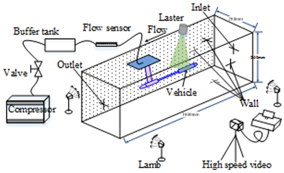
Schematic of test section.

In order to ensure the formation of the ventilated cavitation, the air injection system is used, as shown in Figure 2; the main components include compressor, pressure regulating valve, and flow sensor. In this system, the ventilation pressure and the volumetric flow rate can be measured by the flow sensor.

The test vehicle was mounted in the tunnel. The length of the test body is L = 335 mm, and the diameter is D = 40 mm. A schematic of the test body is shown in Figure 3. During the test, the flow over the test body was at zero angle of attack.

Figure 3.

Cross section of test body and pressure transducer locations.

The surface pressure at different locations on the model was also measured to aid the understanding of the observed flow physics. Seven CYG505 transducers’ conditioner was embedded in the model to facilitate the unsteady pressure measurements. The pressure transducers’ locations are shown in Figure 3. The unsteady pressure signals are sampled at a frequency of 1 kHz. The cavitating flow around the model was imaged with a Photron FASTCAM SA-X high-speed video camera. The resolution of the image was 640 × 144, and the flow was illuminated using three halogen lamps. The frame rate of the video recordings is 3000 frames per second (fps), with a 1/7000 exposure time. Light-emitting diode (LED) phosphors were used as tracer particles; the middle plane was illuminated by an 8-W continuous-wave semiconductor laser (532 nm). A high-speed video camera (Photron FASTCAM SA-X) was used to acquire the images. The camera was operated at 1024 × 632 pixels with a framing rate of 20 kHz, which was sufficient to cover a range of frequencies of interest. The open-source PIV toolbox MatPIV is used to process the velocity vector fields with the interrogation areas of 32 × 32 pixels and 50% overlap in general. The camera and the data acquisition system are triggered manually using the common time.

Results and discussion

The ambient pressure, designated as p₀, is measured using a pressure transducer. The velocity at the inlet of the test section is fixed at U₀ = 8 ± 0.01 m/s, where natural cavitation has not occurred in the velocity.

The ventilated cavitation number, σ, is defined as^20–23

σ = \frac{p_{0} - p_{c}}{0.5 ρ {V_{\infty}}^{2}}

The gas entrainment coefficient is introduced as^21,22

\bar{Q} = \frac{\overset{\cdot}{Q}}{V_{\infty} {D_{n}}^{2}}

The Reynolds number and Froude number are defined as follows

R e = \frac{V_{\infty} D_{n}}{ν}

Fr = \frac{V_{\infty}}{\sqrt{g D_{n}}}

where p₀ is the ambient pressure, p_c is the pressure in the ventilated cavity, ρ is the water density, V_∞ is the mainstream velocity, $\overset{\cdot}{Q}$ is the volumetric gas rate at the pressure p_c, and D_n is the diameter of the axisymmetric body. The ambient pressure, p₀, was 68.4 kPa. The Reynolds number is fixed at 4.04. The Froude number is fixed at $3.2 \times 10^{6}$ . Note that the cavitation number was varied in the range from 0.39 to 0.65 in the experiments by changing the gas entrainment coefficient from 0.05 to 0.15.

Evolution of cavitation pattern and velocity distribution

The experimental evolutions of the ventilated cavitation are shown in Figure 4. In the PIV technology, a thin laser light sheet is used to illuminate the center lengthwise section which shows the detail of cavity interface clearly. Figures 5 and 6 give a typical cavity and the velocity vector distributions in the ventilated cavitation area, respectively. The following is the analysis about the typical cavity shape and its corresponding flow structure.

Figure 4.

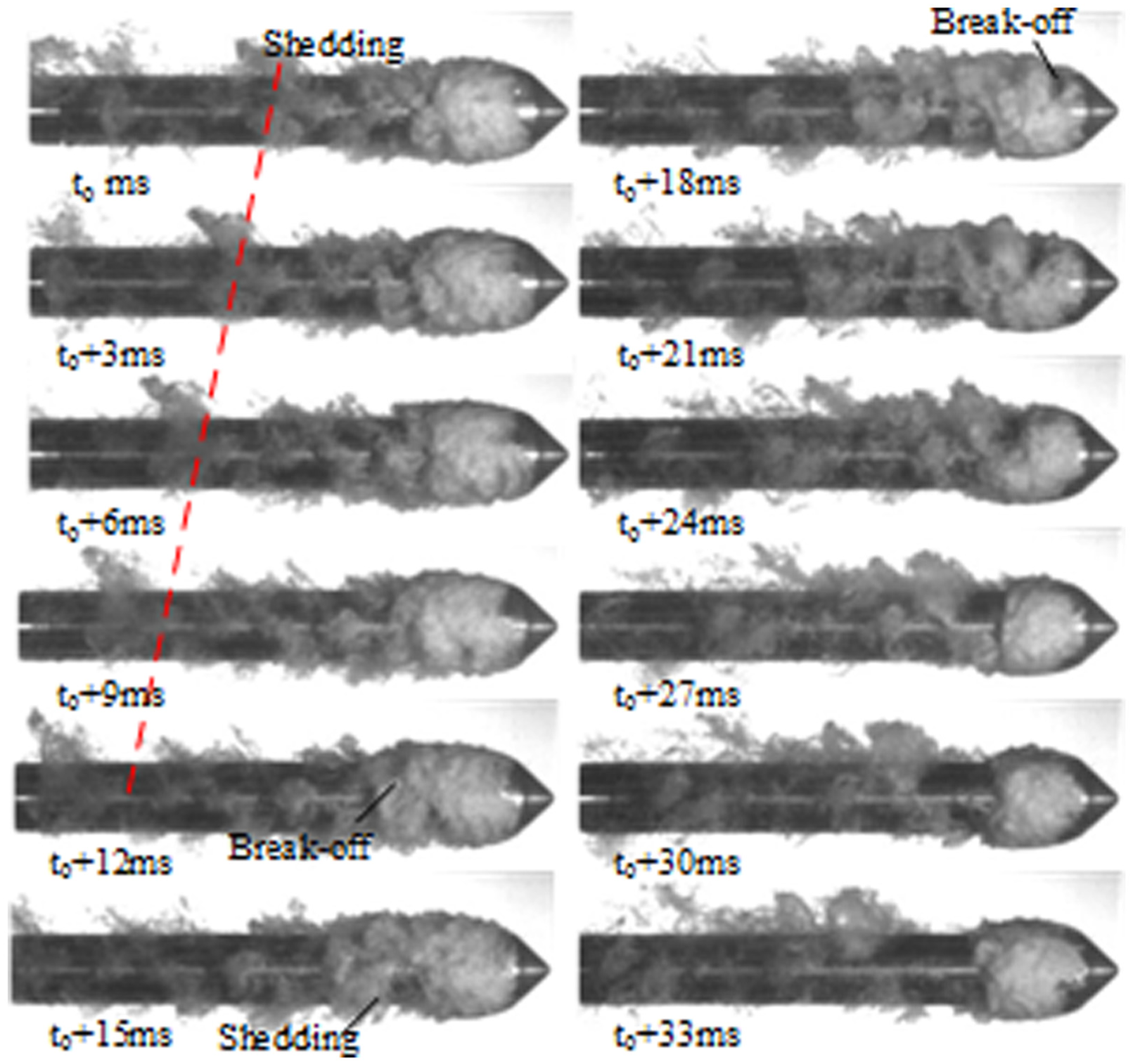
Unsteady cavity shedding process (σ = 0.44).

Figure 5.

Velocity contour and flow streamline.

Figure 6.

Velocity vector.

At the beginning of the cycle, the adverse pressure gradient becomes strong and overcomes the momentum of the flow confined by the near-wall region, and then the re-entrant jet forms. Then the re-entrant jet moves into the cavity after its generation and a partial re-entrant jet motion is observed, as shown in Figure 4.

The forepart of the cavity is transparent in Figure 4 (t₀ − t₀ + 39 ms). The cavity and re-entrant jet influence each other. The unsteady re-entrant jet impinged on the cavity boundaries, and the cavity boundaries become wavy as shown in Figure 4 (t₀ + 19 ms). As the re-entrant jet head flows back, the transparent cavity in front of it is replaced by the opaque cavity gradually at the same time. The shape of the re-entrant jet head is a short curve, as shown by the curves in Figure 4. It can be seen that the re-entrant jet flows back to the forepart of the vehicle with an angle to the vehicle axis; it is because the ventilated cavity is insufficient to overcome the re-entrant jet intrusion. The re-entrant jet moves upstream straightly and curvilinearly. The transparent cavity after the curve is disturbed and generates tiny foam. A closer examination of the opaque regions reveals that the cavity surface is not smooth in these areas. At t₀ + 26 ms, the cavity is cut by this re-entrant jet and forms shedding cavity which is lifted away from the vehicle surface leading to cavity break-off. The short curve moves up to the forepart of the vehicle and the re-entrant jet invades more and more regions till at t₀ + 46 ms when the transparent cavity length in front of it disappears. Then, the vortex structure rotating clockwise forms on the vehicle surface. The vortex distributions and velocity contour can be seen in the interior of the ventilated cavity in Figure 5. From the velocity contour, it is convinced that the cavity area is with low velocity. The low-velocity area is seen in the cavity which represents the vortex as mentioned above. The re-entrant jet rolls back after it reaches the front of the cavity, as shown in Figure 6. The break-off cavity is detached from the vehicle surface, and the break-off behavior becomes violent to cause the shedding cavity to roll up and large cavity vortexes shed toward downstream. Finally, new transparent cavity appears at the shoulder again and repeats the evolution described above. From t₀ + 75 ms to t₀ + 96 ms, the forepart of the transparent cavity has a smooth interface.

Figure 7 shows the evolution of cavity shedding when the cavitation number is 0.65. Similarly, at the beginning, the cavity interface becomes wavy and breaks off. Re-entrant jet appears and moves back to the front of the vehicle under adverse pressure gradient at the closure of the cavity. When the re-entrant jet arrives at the forepart of the vehicle, the cavity separates from the vehicle as a whole, as shown in Figure 7. The shedding bubble flows to the bottom of the vehicle with the main flow. The experimental results show that small cavitation number has a longer cycle and stable time. The reason for the difference is that the cavitation number at 0.44 has smaller influence on the cavity boundaries. It indicates that the cavity break-up may be delayed by the smoother boundaries, compared to cavitation number at 0.65.

Figure 7.

Unsteady cavity shedding process (σ = 0.65).

Wall-pressure fluctuations

Unsteadiness characteristic observed in the cavitation was quantized by measuring the time variation flow properties such as cavity pressure. The locations of the surface pressure sensors are shown in Figure 3. The variation in surface pressure from a high-frequency response transducer was recorded using a high sampling rate data acquisition system, and a sample signal is shown in Figure 8. The flow unsteadiness pressure and the frequency can be calculated using these measurements. Based on the experimental results for the water tunnel vehicle, Figure 12 shows the fast Fourier transform (FFT) of the surface pressure signals for different cavitation numbers.

Figure 8.

Pressure transducer signal for different cavitation numbers: (a) σ = 0.39, (b) σ = 0.41, (c) σ = 0.44, and (d) σ = 0.65.

Cloud cavitation has a regular shedding sequence, as shown in Figure 4. Therefore, the shedding frequency is a distinguishable parameter which depends on the cavitation number, as shown in Figure 4. The shedding mechanism of cloud cavitation is based on the re-entrant jet, and the distance that the jet travels toward the vehicle forepart is an important factor for the shedding frequency. The cavity is cut by this re-entrant jet and the rolling up shedding cavity impinges on the vehicle surface. At this moment, a rapid pressure fluctuation occurs around the impinging position near the vehicle surface.

Figure 8 shows 1-s pressure along the vehicle surface at different cavitation numbers. Four cavitation numbers of 0.39, 0.41, 0.44, and 0.65 are compared. C1–C7 are the vehicle surface pressures and C8 is the test section pressure. The evolution of the cavity causes the change in pressure distribution at the surface of the vehicle. A detailed analysis of the ventilated pressure of different cavitation numbers at pressure sensors (C1–C7) is as follows. When the cavitation number is 0.39, the rear of cavity (C6 and C7) fluctuates heavily around C8 and shedding occurs too. The pressure sensors C1–C5 have lower pressure than pressure sensor C8 as shown in Figure 8(a) because the pressure sensor is in the cavity. There is a small disturbance in the cavity with small irregular pressure fluctuations from C1 to C5, and regular small-scale fluctuations of the surface pressure can be observed at points C6 and C7. With the cavitation number increasing, the fluctuation amplitudes of the pressure sensors C3 and C4 fluctuate with an obvious periodicity. With the increase in cavitation number, the pressure on the surface has different cyclical fluctuations.

Figure 9 shows the evolution of the pressure on the vehicle’s surface in the stage of the cavity breaking off and shedding toward downstream. The right figure is the magnification of the rear part of the left figure which shows pressure wave corresponding to the shedding cavity. A detailed analysis of the ventilated pressure at point C3 is as follows. Initially, the pressure increase is caused by the interaction between the cavity and the vehicle surface as shown in Figures 9(a) and 10(a). Then, the re-entrant jet develops at the closure of the cavity. The interface becomes unstable and the re-entrant jet moves further toward the front. The cavity is cut by this reverse flow as shown in Figure 10(a). The pressure fluctuation decreases gradually at Figure 9(b)–(d). The pressure near the ventilation detected by a pressure transducer is lowest, followed by an increase in pressure fluctuations (see point (e) on Figure 9).

Figure 9.

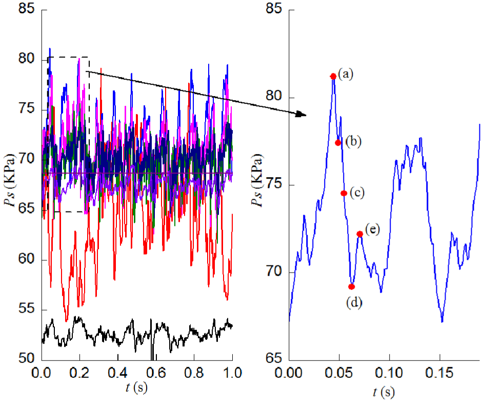
Pressure transducer signal for σ = 0.44.

Figure 10.

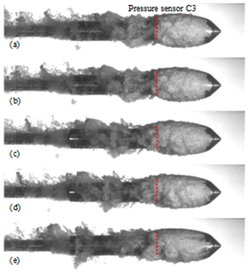
Time evolutions of cavity (σ = 0.44).

The average pressure of 1 s along the vehicle surface was estimated and the pressure fluctuations for different cavitation numbers are depicted in Figure 11. Here, Ps represents the pressure on the vehicle surface, D is the diameter of the axisymmetric body, and x is the distance between the head of model and the pressure sensor. The pressure experiences the adverse pressure gradient at the rear part of the cavity. The pressure is accompanied by an increase in the intensity of pressure fluctuations. Then the pressure near the ventilated cavity decreases. As shown in Figure 11, the pressure which is in the rear part of the cavity location increases with the decrease in the cavitation number.

Figure 11.

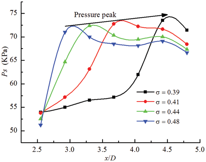
Time-averaged wall-pressure distribution.

Shedding frequency

The characteristic frequency of the variation is obtained by taking the FFT of surface pressure signals. From the FFT, frequencies corresponding to the maximum Fourier domain amplitude were identified as dominant frequencies. Figure 12 shows FFT of pressure signal normalized by the maximum Fourier magnitude. The characteristic frequency is low and the fluctuation characteristics vary with different cavitation numbers, which is due to the variation in the unsteady cavities. When the cavitation number is 0.39, cavity sheds downstream periodically in the cavitating flow and irregular fluctuations of the surface pressure can be observed in C6 and C7. To explain the shedding cavity frequency, Figure 12 shows some statistical results based on 1-s pressure data for four different cavitation numbers. From the results and analysis above, when σ = 0.44, the dominant frequency is 10.99 Hz. The fluctuation amplitude near the rear part of the cavity (Figure 12(b), C4) is much larger than that of other pressure sensors (Figure 12(b), C5–C7). The low characteristic frequency corresponds to the inherent fluctuation frequencies of the cavitating flow. When σ = 0.39, σ = 0.41, and σ = 0.65, the dominant frequency values are 7.57, 9.52, and 21.6 Hz.

Figure 12.

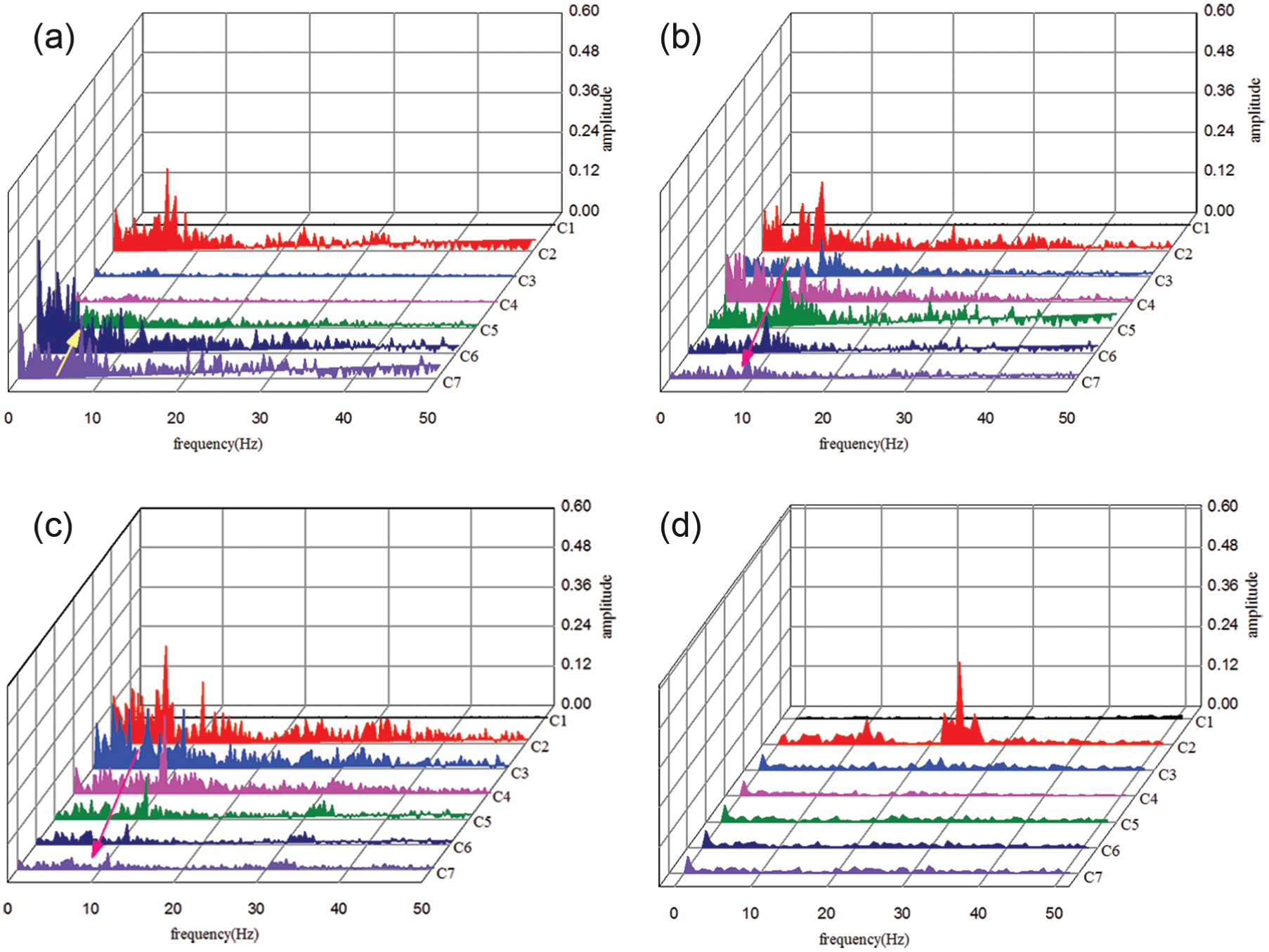
FFT of the pressure signal normalized by maximum Fourier space magnitude: (a) σ = 0.39, (b) σ = 0.41, (c) σ = 0.44, and (d) σ = 0.65.

The non-dimensional dominant frequency is $St = fD / U_{\infty}$ . f represents the frequency of shedding and σ represents the cavitation number that depends on the gas entrainment coefficient. If we change the ambient pressure while maintaining the gas entrainment coefficient, the different ambient pressure gave basically the same Strouhal number as shown in Figure 13. With the reduction in the cavitation number, the dominant frequencies of the pressure signal decrease which corresponds to cavity shedding cycle. The dominant frequencies are compared with the results obtained by other researchers as shown in Figure 14. The difference in the values of growth rate about dominant frequencies in Figure 14 may be caused mainly by the model design, cavitation number, and scale effects, and it is the ventilated cavitation in this experiment instead of the natural cavitation experiment in Chen et al.²⁴

Figure 13.

Non-dimensional dominant frequency with cavitation number.

Figure 14.

Dominant frequency of ventilated and natural cavitation.

Conclusion

In this study, some aspects of the flow physics of a ventilated vehicle are experimentally investigated in the high-speed water tunnel. The mechanism of ventilated partial cavitations can be clearly observed through the image analysis based on the high-speed video observation and wall-pressure measurements. As a result, the following conclusions can be drawn:

The periodically shedding cavities are chosen for further exploration of cavitation shedding dynamics and associated flow features. A partial re-entrant jet motion is observed. As the re-entrant jet head flows back, the transparent cavity in front of it is replaced by the opaque cavity gradually at the same time. The re-entrant jet flows back to the forepart of the vehicle with an angle to the vehicle axis. The cavity area where the vortex structure forms is with low velocity.

The pressure signals for different cavitation numbers are depicted, and the average pressure of 1 s along the vehicle surface was estimated. The evolution of the cavity causes the change in pressure distribution at the surface of the vehicle. A fluctuant pressure peak is located at the cavity closure depending on the cavitation number. The pressure peak increases with the decrease in the cavitation number.

Based on pressure transducer measurements, it is found that for the case of transitory cavity re-entrant jet-induced shedding, the main factor for the pulsation is mainly caused by periodic shedding of large-scale vortex cavities at the rear region of the cavity. With the reduction in the cavitation number, the presence of dominant frequencies of the pressure signal decreases which corresponds to cavity shedding cycle.

Footnotes

Academic Editor: Pietro Scandura

Declaration of conflicting interests

The author(s) declared no potential conflicts of interest with respect to the research, authorship, and/or publication of this article.

Funding

The author(s) disclosed receipt of the following financial support for the research, authorship, and/or publication of this article: This work was supported by the Natural Science Foundation of Heilongjiang Province of China (grant no. A201409). Their financial support is gratefully acknowledged.

References

Rouse

Mcnown

JS.

Cavitation and pressure distribution: head forms at zero angle of yaw. Iowa: State University of Iowa, 1948.

Arakeri

Acosta

AJ.

Viscous effects in the inception of cavitation on axisymmetric bodies. J Fluid Eng 1973; 95: 519–527.

Ceccio

Brennen

CE.

Dynamics of attached cavities on bodies of revolution. J Fluid Eng 1992; 114: 93–99.

Vlasenko

. Experimental investigation of supercavitation flow regimes at subsonic and transonic speeds. In: Proceedings of the fifth international symposium on cavitation, Osaka, Japan, 1–5 November 2003, Cav03-GS-6-006, pp.1–8.

Chen

. Numerical investigation on the cavitation collapse regime around the submerged vehicles navigating with deceleration. Eur J Mech B: Fluid 2015; 49: 153–170.

Stutz

Reboud

JL.

Experiments on unsteady cavitation. Exp Fluids 1997; 22: 191–198.

Huang

Wang

GY.

Experimental and numerical investigation of unsteady cavitating flows through a 2D hydrofoil. Sci China Technol Sci 2011; 54: 1801–1812.

Huang

Young

Wang

. Combined experimental and computational investigation of unsteady structure of sheet/cloud cavitation. J Fluid Eng 2013; 135: 071301.

Wang

Huang

. The inception cavitating flows over an axisymmetric body with a blunt head-form. J Hydrodyn 2015; 27: 359–366.

10.

Wang

Chen

. Three-dimensional unsteady cavitating flows around an axisymmetric body with a blunt headform. J Mech Sci Technol 2015; 29: 1093–1101.

11.

Wang

Huang

Experimental investigation on cavitating flow shedding over an axisymmetric blunt body. Chin J Mech Eng 2015; 28: 387–393.

12.

Wang

Huang

. Shedding phenomenon of ventilated partial cavitation around an underwater projectile. Chin Phys Lett 2012; 29: 014601.

13.

Huang

. Study of characteristics of cloud cavity around axisymmetric projectile by large eddy simulation. J Fluid Eng 2014; 136: 051303.

14.

Wang

Liao

. A study on the collapse of cavitation bubbles surrounding the underwater-launched projectile and its fluid–structure coupling effects. Ocean Eng 2014; 84: 228–236.

15.

Ceccio

SL.

Friction drag reduction of external flows with bubble and gas injection. Annu Rev Fluid Mech 2010; 42: 183–203.

16.

Wosnik

Schauer

Arndt

. Experimental study of a ventilated supercavitating vehicle. In: Proceedings of the fifth international symposium on cavitation, Osaka, Japan, 1–5 November 2003, Cav03-GS-6-006, pp.1–4.

17.

Savchenko

Supercavitation—problems and perspectives, 2001, http://resolver.caltech.edu/cav2001:lecture.003

18.

Rashidi

Pasandideh-Fard

Passandideh-Fard

. Numerical and experimental study of a ventilated supercavitating vehicle. J Fluid Eng 2014; 136: 101301.

19.

Wang

Huang

Wang

. Experimental and numerical investigation of ventilated cavitating flow with special emphasis on gas leakage behavior and re-entrant jet dynamics. Ocean Eng 2015; 108: 191–201.

20.

Birkhoff

Jets, wakes, and cavities. New York, NY: Academic Press, 1957.

21.

Logvinovich

GV.

Hydrodynamics of flows with free boundaries. Kiev: Naukova Dumka, 1969, p.128.

22.

Epshtein

LA.

Methods of theory of dimensionality and similarity in problems of ship hydromechanics. Leningrad: Sudostroenie Publishing House, 1970.

23.

Knapp

Daily

Hammitt

FG.

Cavitation. New York: McGraw-Hill, 1970.

24.

Chen

Wang

. Observations and measurements on unsteady cavitating flows using a simultaneous sampling approach. Exp Fluids 2015; 56: 1–11.

Experimental investigation of unsteady characteristics of ventilated cavitation flow around an under-water vehicle

Abstract

Keywords

Introduction

Experimental setup

Results and discussion

Evolution of cavitation pattern and velocity distribution

Wall-pressure fluctuations

Shedding frequency

Conclusion

Footnotes

Declaration of conflicting interests

Funding

References