Sage Journals: Discover world-class research

Abstract

This research proposes an innovative model for calculating the temperature distribution of a composite pulley inside a belt drive. The main advantage of the proposed model is a significant reduction in the costs of calculation resources and time. This model adopts two classical theories to determine the heat generation flux and subsequent thermal flow into the pulley. Then, ordinary differential equations are developed in this model according to the irregular geometric structures of a pulley to describe the thermal flow inside this component. Afterward, analytical solutions of the ordinary differential equations are derived to provide final temperature distributions of the pulleys. Moreover, measurements of thermal properties are conducted to reduce the influence of errors. To improve the reliability of the results, experimental temperature measurements were performed on a composite pulley of a designed belt drive system in an engine dynamometer system to validate this analytical model under various operating conditions. The temperature data measured at multiple locations indicate good agreement with the corresponding analytical results. Therefore, the temperature distribution provided by this model can be utilized for the development of high-thermal resistance composite. It can also be used for thermal fatigue simulations of composites under numerous load cases.

Keywords

Analytical thermal model thermal behavior fiber-reinforced plastic pulley front-end accessory drive

Introduction

The front-end accessory drive (FEAD) system is a common powertrain form in various industries ranging from the automotive industry to the oil and gas industry. One current prospect for belt drives involves the use of fiber-reinforced plastic (FRP) to replace the conventional steel alloy as the pulley material. Using an FRP composite offers remarkable advantages such as cost-effectiveness, corrosion avoidance, lightweight, and robustness. However, the remarkable amount of heat generated within the engine¹ also increases the under-the-hood temperature, making FRP pulleys work under an elevated-temperature environment. In addition, the low thermal conductivity and heat dissipation coefficient of FRP may cause excessive operationally generated heat to accumulate inside the pulley, resulting in deterioration and blistering of the pulley surface. This article considers an FRP pulley in a FEAD, as shown in Figure 1, for a vehicle engine as an example belt drive system because of the large amount of heat generated within the system and the high ambient temperature around the vehicle engine. Then, an investigation is presented into the thermal generation and thermal flow behaviors within the system, enabling the creation of a thermal model based on the pulley structure and, ultimately, the prediction of the accurate temperature distribution on the structure surface in a timely manner. This model is beneficial to designers for use in predicting temperatures and developing a suitable thermal-resistant FRP material to avoid thermal failure according to the basic belt layout sketch in the early design stage. This approach is time-efficient and can be used to provide input information for the thermal fatigue analysis of FRP composites under numerous engine operating conditions. In addition, the approach can be integrated with other commercial analytical algorithms such as vibration analysis, enabling designers to consider all aspects of a belt drive system’s design.

Figure 1.

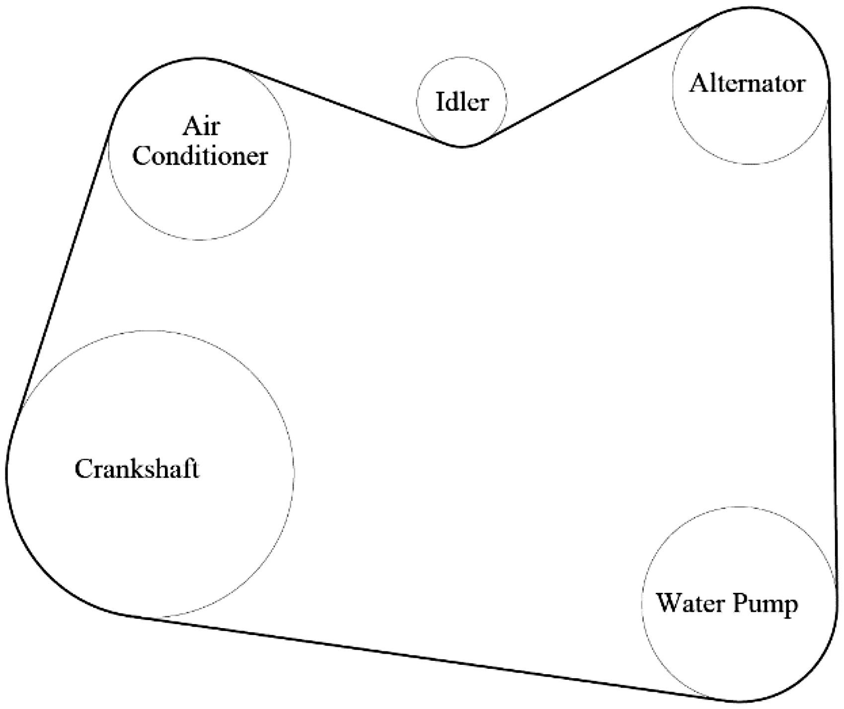
Schematic of an FEAD system.

To estimate the pulley thermal temperature, this thermal model, as with other general thermal procedures, is developed by integrating three separate research fields: (1) heat generation in the belt drive system, (2) heat partitioning at the belt-pulley engaged surface, and (3) heat transfer within the pulley. As governed by the first law of thermodynamics, the belt drive power loss algorithm can be used to estimate the heat generation in the belt drive system. Here, power losses in the system are transformed into heat and dissipated into the environment. The initial research in this area used a mathematical algorithm to calculate the power loss during flat and V-belt transmissions by analyzing the pressure distribution along the surface at the outer radius of the pulley, belt deformations, and belt-pulley slippage.² Manin et al.³ expanded the theory to a multipulley V-ribbed belt drive system. In addition, an analytical approach was used to develop a power loss model for a rubber V-belt continuously variable transmission (CVT) by considering circumferential slipping as the primary energy loss.⁴ Another algorithm of power losses based on belt rubber hysteresis losses was developed and validated by dynamic mechanical analysis (DMA) experiments.^5,6 This study also considered the additional belt-pulley slipping and power loss from bearings to construct a full-scale power loss model of the belt drive system for industrial use.⁷ Moreover, several factors have impacts on the power losses. The influence of the operating parameters on the speed loss has been investigated in a previous study.⁸ Qin et al.⁹ developed an analytical model for the friction damping of round clamp band joints, which can predict the energy dissipation caused by the friction contact between the joint components. In addition, a study focused on power loss was conducted through experiments. A dynamic model was developed based on the experiments to achieve the optimal efficiency of rubber-belt CVTs by instantly adjusting the axial forces on the pulleys.¹⁰

Regarding the heat partitioning stage, heat partitioning theories for pad-disk or pin-disk applications are applicable for the heat partitioning for the application of belt-pulley engagements. Some theoretical models of heat partitioning for sliding contact surfaces that use the heat source method. Analytical algorithms (both transient and quasi-steady-state) have been developed to determine the temperature rise distribution due to frictional heat sources at the interface for the classical case of a tribological sliding system.¹¹ One study also developed general analytical solutions for the temperature rises associated with different shapes of contact surfaces and heat intensity distributions using Jaeger’s classical heat source method for the classical case of a tribological sliding system.^12,13 A three-dimensional (3D) theoretically and experimentally analytical model has been established to calculate the heat partition coefficient and surface temperatures in a pin-on-disk application.¹⁴ A study developed an analytical-numerical model to predict the temperature distribution of a braking system consisting of a pad and disk.¹⁵ Vick and Furey¹⁶ presented a theoretical calculation for the temperature rise at interacting surfaces for a multiple-sliding contact application. In addition, in another work, researchers applied the displacement gradient circulation method to perform thermal-structural coupling analysis for a brake friction pair during its operating process.¹⁷ In addition, other studies have focused on parameters that influence the heat partitioning coefficient at the engaged surface. One study investigated the influence of several parameters, including the relative velocity between two contacting components with surface roughness, on heat partitioning and the surface temperature at the sliding contact surfaces.¹⁸ Another study focused on the temperature profile and frictional heat flux density distribution of dry friction under various sliding velocities between two rough-contact asperities.¹⁹ Nosko²⁰ investigated and developed a solution for calculating the heat partitioning coefficient and surface temperature at sliding semispaces with the consideration of contact heat exchange and adhesion-deformational heat generation.

For the stage of heat transfer for pulleys, there has been a large amount of research in heat transfer analysis for round-shaped components. Green’s function was used to solve the governing heat equations derived by considering various operating parameters of a disk brake system.²¹ Conjugate computational fluid dynamics (CFD) was adopted to perform heat transfer analysis of a rotational disk rotor.²² Some research has used heat transfer analysis for design and other applications. The numerical CFD approach was used to perform thermal analyses of different vane-shaped disk brake rotors.²³ Two ventilated brake disks were compared to investigate the effects of cross-drilled holes on the heat transfer and fluid flow of disks.²⁴ A study presented steady-state and transient heat transfer analyses of functionally graded cylinders reinforced with carbon nanotubes using a meshless method.²⁵ A similar study also focused on the heat transfer and mechanical analyses of nanocomposite thick cylinders reinforced with graphene using the mesh-free method.²⁶ Another study examined the thermal and stress wave propagation behaviors of sandwiched plates with carbon nanotube-reinforced face sheets.²⁷ Additional research used commercial software to investigate the influences of three types of cast iron and the braking mode on the thermal behavior of a full and ventilated brake disk.²⁸ Further research used a transient numerical method to determine the thermal effects of a circular oil jet impinging on a reciprocating disk subjected to a uniform wall heat flux using the volume of fluid (VOF) method.²⁹ Moreover, there is some literature specifically focusing on the heat transfer coefficients of rotational bodies. Pellé and Harmand³⁰ experimentally examined the effect of an axial cooling inflow on the local heat transfer of a rotor surface in a discoidal rotor-stator system for the application of an electrical wind generator. Lallave and Colleagues^31,32 demonstrated that the local heat transfer coefficient on a rotating and uniformly heated solid disk was influenced by several parameters, such as the turbulence intensity and rotational rate.

The above literature provides the research background related to this pulley thermal mode. Alternatively, some research has focused on other methods to provide the temperature distribution of pulleys and belt drive systems. An analytical algorithm was presented for a two-pulley-one-belt drive system.² This algorithm, which idealizes pulleys as round cylinders and the belt as a flat layer, can provide the temperature distribution of a basic two-pulley-one-belt system. Other research has focused on numerical methods. Wurm et al.^33,34 integrated the zone-averaging method into a numerical algorithm and developed an experimentally validated approach by which to analyze the thermal analysis of a continuous variable transmission and predict the pulley temperature.

Nonetheless, the available research is not ideal for rapidly predicting accurate temperatures of pulleys. The current numerical method requires substantial computational resources and long solution periods. The numerical method developed by Wurm et al.³⁴ requires hours for each case and is not suitable for temperature prediction when modeling a large number of engine operating conditions. The current analytical method oversimplifies the geometries and features of components, significantly reducing its ability to provide accurate results. Therefore, to achieve efficient temperature predictions, this article adopts an innovative analytical algorithm that provides comparable accuracy to that of common numerical approaches alongside a significant decrease in the simulation time. In addition, the algorithm takes into account the actual structure of the pulley to achieve an accurate prediction of its temperature. Moreover, to reduce the influence of measurement error, input parameters are measured through experiments according to industrial standards. Finally, this article also includes validation experiments for this analytical temperature model to guarantee its ability to deliver accurate temperature predictions.

Pulley thermal analytical model

This model investigates the thermal behavior within the pulley and the rest of the belt drive system and establishes a set of innovative thermal ordinary differential equations (ODEs) that consider the heat dissipation based on the general complex structures of the pulley. Moreover, it provides analytical solutions for these equations to predict the pulley temperature accurately and efficiently. The whole approach constitutes the pulley thermal analytical model.

Overall calculation process

The calculation procedure of the thermal model is divided into three steps, and its workflow is shown in Figure 2. The first step is to determine the heat generation flux within the system. The second step is to use the band contact algorithm³⁵ to calculate the heat flux flowing into the pulley by determining the heat partition coefficient ξ at the belt-pulley interface. The next step is to perform a thermal analysis of the pulley, and the third step is to calculate the heat distribution of the investigated pulley based on the heat flow and dissipation on the pulley. Finally, the predicted temperatures at selected locations on the pulley surfaces are outputted.

Figure 2.

Single pulley model.

In this section, section “Determining the heat source information in the pulley system” develops the calculation of heat generation in the belt drive system. Section “Determining the heat partition coefficient” introduces a heat partition coefficient to determine the heat flux flowing into the pulley. Section “Pulley internal thermal analysis” presents the establishment of algorithms to calculate the temperature of a selected pulley.

Determining the heat source information in the pulley system

The heat source is primarily the power losses of the high-speed FEAD operation. During the belt and pulley movement, five forms of power losses exist, and all of them are transformed into heat. The first four types, which are belt bending, belt stretching, belt shearing, and belt radial compression (Table 1), are the belt internal power loss P_h. These power losses generate heat inside the belt. The last type, which is belt-pulley slipping (Table 1), is the contact surface power loss P_f.

Table 1.

Classification of power losses

Power loss type	Schematic
Belt bending
Belt radial compression
Belt tension
Belt shearing
Belt-pulley slipping

However, this research considers only the heat from the contact surface power loss as the main source in the thermal analysis. The belt internal power loss contributes only 20%–30% of the total power losses from all five modes, because the frictional heat generated on the pulley-belt surface is much greater than the energy loss through the belt rubber deformation caused by belt bending, stretching, shearing, and radial compression. Moreover, the heat transformed from this power loss is inside the belt. Because the belt surface areas exposed to the environment are much larger than the belt-pulley contact areas, most of this heat dissipates into the environment through the exposed surface during the high-speed operation. Therefore, the contact surface power loss is considered the only heat source in this research.

The calculation of the frictional heat flux depends on the belt wrap force and speed differential between the pulley and the belt²

P_{f} = \int_{0}^{a} μ p (α) v d φ

(1)

where

μ

is the frictional coefficient, α is the wrap angle, p is the belt pressure distribution on the belt-pulley engaged surface, v is the pulley-belt sliding speed, and dφ is an infinitesimal angular element of the wrap angle.

Determining the heat partition coefficient

This step is performed to determine the percentage of the heat flux generated in the previous step that flows into the pulley and provide this information for use in the pulley inner thermal analysis in the next step. At the belt-pulley contact surface, there are two simultaneous phenomena, which are the frictional heat generation and the heat exchange between the belt and the pulley. To be specific, the generated frictional heat flows into both the pulley and the belt, causing different temperature increases at the two sides of the belt-pulley contact surface, followed by heat exchange between the two components. However, the difference in the elevated temperatures at the two sides of the contact surfaces is less than the temperatures increase from the ambient temperature, indicating that the exchanged heat flux is not significant compared with the heat generation from belt-pulley slip. Therefore, this study focuses on only the frictional heat partitioning without consideration of the heat exchange, and the influences of the temperature effect and thermal behavior of the belt on the calculation of this heat partitioning are not considered.

During the operation, the belt and pulley have a relative sliding velocity v to each other. If the belt is defined as a stationary reference, the pulley can be considered to be rotating against the belt at speed v. Then, this phenomenon can be idealized as a pad sweeping against an infinitely long plate, and the band contact used to calculate the heat partition coefficient for the pad-on-disk friction can be applied for the belt-pulley contact³⁶

ξ = 1 - \frac{1}{1 + \frac{λ_{b}}{λ_{p}} \sqrt{1 + P e}}

(2)

where λ_p and λ_b are the thermal conductivities of the pulley and belt, respectively;

P e = (v W_{d} / 2 κ_{b})

is the Péclet number; W_d is the belt width, with a standard value of 0.0024 m; and κ_b is the thermal diffusivity of the belt, which is 0.12 m²/s. The belt speed is less than 35.6 m/s, and the range of the slip rate is from 0.5% to 2.5% under industrial operating conditions, resulting in a negligibly small Pe value of approximately 0. Then, the heat flux entering the pulley per second Φ _p is reduced to

Φ_{p} = \frac{λ_{p} P_{f}}{λ_{p} + λ_{b}}

(3)

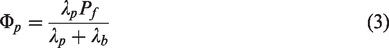
Moreover, because there is no heat source inside the pulley,² the heat flowing into the pulley is the same as the heat dissipated on the pulley surfaces. Therefore, Φ _p is also considered the total heat dissipation from the pulley surfaces.

Pulley internal thermal analysis

This analysis uses the heat flux Φ _p entering the pulley to calculate the thermal flow and dissipation for the pulley. The industrial pulleys used in the FEAD follow the universal simplified geometry with various dimensions for different sizes of pulleys, as shown in Figure 3. This configuration consists of top and bottom flanges connected by a middle web and strengthened by fins on two sides. This research creates a pulley thermal model to calculate the thermal flow and temperature distribution based on this general structure.

Figure 3.

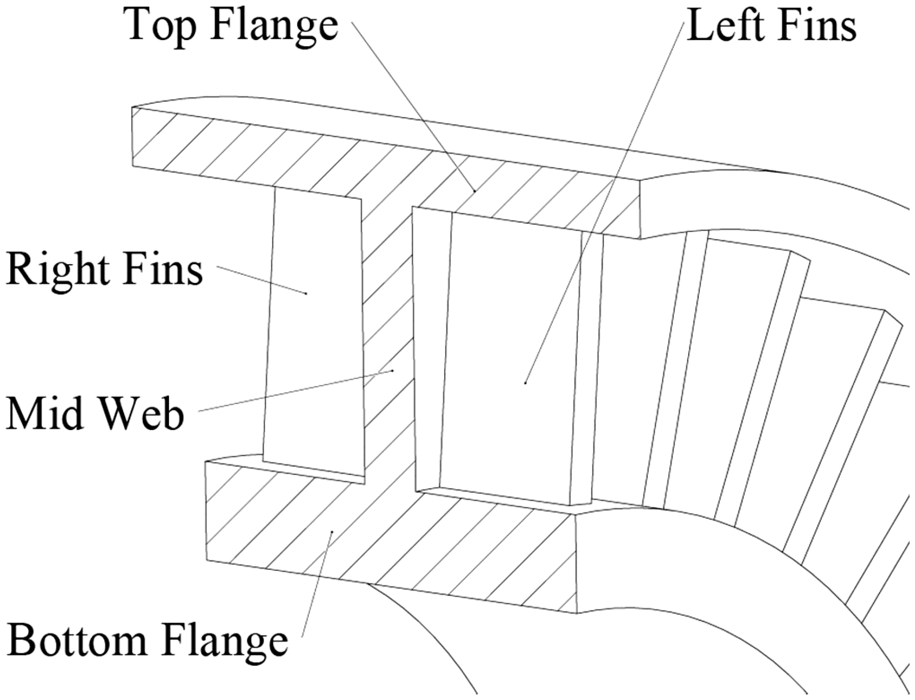
Structure of a general simplified pulley in the FEAD system.

The procedure for predicting the pulley temperature profile is not straightforward because the temperature distribution cannot be acquired directly from Φ _p . A simple workflow is presented here. The analysis first assumes that the temperature at one location is known. In this research, the temperature at the outer radius of the pulley T_p is selected and considered an assumed value of ${T^{'}}_{p}$ . Then, an analytical model is established according to the pulley geometry to calculate the assumed temperature distribution on the pulley surfaces. Next, using the integration from the outer to inner radius of the pulley, the procedure calculates the assumed total heat dissipation from the pulley surfaces to the environment ${Φ^{'}}_{p}$ according to the surface temperature and ambient temperature T_a. In the last step, this model corrects $T^{'} (r)$ to output the final temperature at the pulley surface T(r) according to the ratio of ${Φ^{'}}_{p}$ and Φ _p from equation (3).

The following is a detailed illustration of this analysis, which has the preliminary purpose of helping create an analytical model based on the complex pulley structure. The preliminary assumption is that the temperature variation along the pulley axial direction can be neglected at both the top and the bottom flanges. Both flanges are thin layers that are exposed to either the belt or the shaft, with a constant high temperature on one side and a constant low ambient temperature on the other side. This condition results in a temperature gradient in the pulley radial direction but uniformity in the axial direction. The web in the middle requires some preliminary analysis. It has a minimal thickness in the radial direction, leading to negligible temperature variation in this direction. In contrast, this preliminary assumption does not apply to fins because each fin has a very large area exposed to the environment, resulting in a substantial temperature gradient in the pulley axial direction.

The next step is to build a thermal model based on the pulley structure. This thermal model uses variables (L₁ … L₃, R₁ … R₄ in Figure 4) to represent all dimensions of the pulley because the structure is complex and because the distances vary with different pulleys. The model first considers the I-shaped continuous round structure and then incorporates the fins. The I-shaped structure is divided into three layers as shown in Figure 4 for thermal model creation. Then, every layer is assumed to have a continuous rectangular cross section. Taking one dashed area as an example, the heat balance can be established (Figure 5) as

2 π λ_{p} \cdot 2 L_{i} \frac{d}{d r} (r \frac{d T}{d r}) d r = 2 h (T - T_{a}) \cdot 2 π rdr

(4)

where 2L_i is the width of the dashed area of the ith investigated layer (with 2L_i used for easy calculation and equation derivations) and h is the heat transfer coefficient on the pulley surfaces. The function T(r) describes the temperature distribution along the radial direction.

Figure 4.

Structure of a general pulley in the serpentine belt system.

Figure 5.

Thermal behavior at one round section.

To acquire T(r), equation (4) can then be translated into an ODE

\frac{d^{2} T}{d r^{2}} + \frac{1}{r} \frac{d T}{d r} - \frac{h}{L_{i} λ_{p}} (T - T_{a}) = 0

(5)

However, the heat dissipation on the large surfaces of the fins dramatically increases the temperature gradient from the outer diameter to the inner diameter of the connected web along the pulley radial direction, making it such that equation (5) must account for the influence of the fin thermal dissipation on the heat distribution of the web. To this end, an integration method is used. In a differential increment dr of Layer 2 (Figure 6), the heat flux through the surface A_f to the fins is equal to the total heat flux dissipated on the fin surfaces, while the heat flux through the pink surface is the only heat dissipation mode on that surface. It is obvious that the surfaces of the fin are larger than the pink area, corresponding to the heat loss on the green surface being several times higher than that of the pink area. This work introduces a coefficient η_f and uses hη_f to represent the heat dissipation increased by the fin η_f times on the green surface compared to the pink area. The total dissipation rate on one side of the round differential increment is (hNW_bdrη_f + h(2πrdr − NW_bdr)), while the dissipation rate is 2hπrdr when no fin is attached. Therefore, the heat dissipation is increased by a factor of (1 + NW_bL_f(η_f − 1)/2πr), and equation (5) is updated to

\frac{d^{2} T}{d r^{2}} + \frac{1}{r} \frac{d T}{d r} - \frac{[1 + N W_{b} (η_{f} - 1) / 2 π r] h}{L_{i} λ_{p}} (T - T_{a}) = 0

(6)

Figure 6.

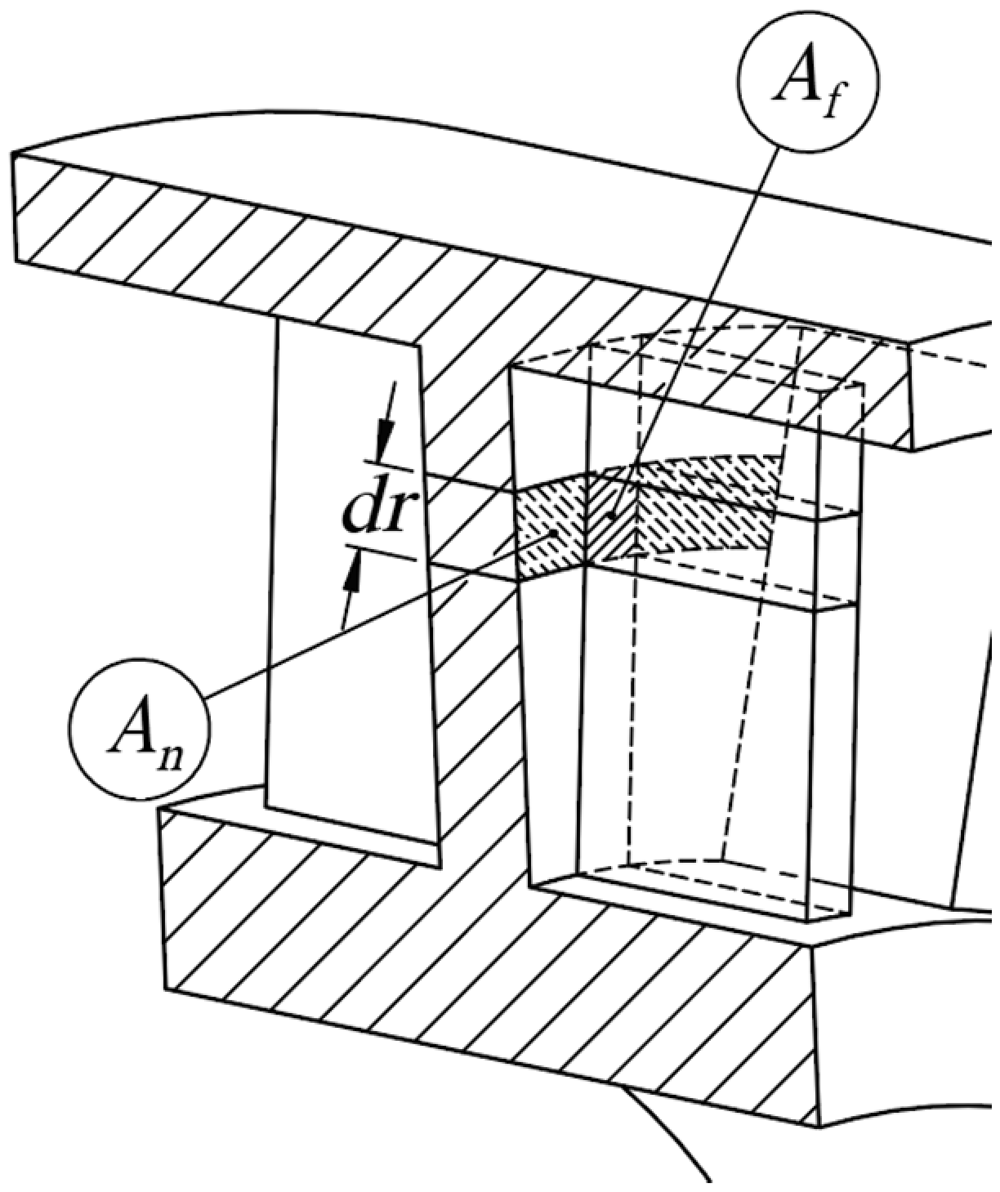
Two areas with and without a connection to a fin.

Equation (6) is applicable to all three layers. In Layers 1 and 3, owing to the lack of augmentation of heat dissipation by the fins in both flanges, η_f is 1 in equation (6), which makes the equation equivalent to equation (5). In Layer 2, the temperature distribution can be acquired from equation (6) when the value of η_f is calculated.

The calculation procedure of η_f in equation (6) is to acquire the temperature distribution and the heat flux dissipated on the fin surfaces and divide the heat flux dissipated without a fin section to obtain the incremental ratio. Taking one differential increment dx of Layer 2 to perform the analysis (Figure 6), the fin on one side of the pulley can be treated as a rectangle bar. The temperature decreases from the web surface to the fin edge due to heat dissipation on the fin surfaces. The balance of heat in this small plate is³⁷

\frac{\partial^{2} S}{\partial x^{2}} = - \frac{2 h d r (S - T_{a})}{λ_{p} A_{f}} = - \frac{2 h (S - T_{a})}{λ_{p} W_{b}}

(7)

where A_f is the web-fin bonded area shown in Figure 6. The function S(x) represents the temperature distribution on the fin element along the pulley axial direction; hence, S(0) is the temperature on the web surface at radius r, which equals T(r); S(L_b) is the temperature at A_e in Figure 7, the edge surface of the fin; and L_b is the fin length on one side of the pulley.

Figure 7.

Geometry of the fin.

The analytical solution of equation (7) in the range from 0 to L_f provides the temperature distribution on this infinitesimal element dr, which is

{\begin{cases} S (x) = \frac{[S (0) - T_{a}] \cosh [z \cdot (L_{b} - x)]}{\cosh (z \cdot L_{b})} + T_{a} \\ z = \sqrt{\frac{2 h}{λ_{p} W_{b}}} \end{cases}

(8)

The total surface heat dissipation rate is calculated by integrating the heat dissipation on the surfaces according to the temperature provided by equation (8), as shown in the following equation

Φ_{fin} = Φ_{f s} + Φ_{f e} = \int_{0}^{L_{f}} 2 h d r \cdot S (x) d x + h A_{e} [S (L_{f}) - T_{a}]

(9)

η_f, which is the ratio of the total heat dissipation of a differential section of the fin to the natural heat dissipation of area A_f, can be calculated as

η_{f} = \frac{Φ_{fin}}{Φ_{A f}} = \frac{\int_{0}^{L_{f}} 2 \cdot S (x) d x}{W_{b} \cdot [G (0) - T_{a}]} + \frac{G (L_{f}) - T_{a}}{G (0) - T_{a}}

(10)

Equations (6) and (10) provide thermal governing equations to describe the heat flow behavior of each layer within the pulley, and then the temperature distribution of a layer T(r) is obtained through the integration of equations (6) and (10) from the outer radius to the inner radius of this layer.

Note that the heat dissipation coefficient η_f varies at different pulley radial distances from its center during the calculation (Figure 8). The dramatic changes at different relative airspeeds caused by the same angular velocity but different radial distances indicates that the pulley’s local heat dissipation coefficient at different radii is not uniform.³⁸ Moreover, the hollow space between two fins also generates intensive flow turbulence around the pulley during its high-speed operation. However, to provide an efficient solution, this model does not consider this excessive turbulence and considers only the h_p is a function of the local relative air angular velocity.

Figure 8.

Different tangential speeds.

Therefore, the relationship between h_p and the local relative air angular velocity ω_pr is represented by a second-order polynomial as

h = k_{h} ω_{p}^{2} r^{2} + p_{h} ω_{p} r + q_{h}

(11)

where k_h, p_h, and q_h are the three coefficients. To ensure the high accuracy of the thermal model, this work integrates equation (11) into equation (6) to provide a new equation

\frac{d^{2} T}{d r^{2}} + \frac{1}{r} \frac{d T}{d r} - \frac{[a_{T} r^{2} + b_{T} r + c_{T}]}{d_{T}} (T - T_{a}) = 0

(12)

where

\begin{array}{l} a_{T} = k_{h} ω_{p}^{2} \\ b_{T} = p_{h} ω_{p} + Λ_{f} k_{h} ω_{p}^{2} \\ c_{T} = (Λ_{f} p_{h} ω_{p} + q_{h}) + Λ_{f} q_{h} r^{- 1} \\ d_{T} = L_{i} λ_{p} \\ Λ_{f} = \frac{N W_{b} (η_{f} - 1)}{2 π} \end{array}

Equations (10) and (12) do not have a direct analytical solution; however, two modifications can achieve such a solution. The first is using a uniform h for z in equation (8) to make η_f constant. During the solution of equations (10) and (12), h is a function of r and is associated with the η_f variable in equation (10) at different radial distances, but the fluctuation of η_f at the range from the outer radius to the inner radius can be neglected because both the nominator and denominator in equation (8) include z, which includes h, reducing the influence of the variation on η_f. Then, an averaged value of h is used in equation (8). The second modification is using a constant r for $Λ_{f} q_{h} r^{- 1}$ in c_T of equation (12) because $r^{- 1}$ in c_T gives the least change compared with other higher-order terms such as $a_{T} r^{2}$ and $b_{T} r$ in equation (12). Upon replacing r with the average radius of the investigated layer, (R_m + R_n)/2, gives

c_{T} = (Λ_{f} p_{h} ω_{p} + q_{h}) + 2 Λ_{f} q_{h} / (R_{m} + R_{n})

(13)

With these treatments, equation (12) becomes a kind of Heun’s equation,³⁹ for which an analytical solution is available. Upon applying the boundary condition stating that $T (R_{n}) = limited$ (the temperature at R_n is finite), the analytical solution of equation (12) for one layer is

{\begin{cases} T (r) = \frac{e^{g (r)} \cdot f (r)}{e^{g (R_{m})} \cdot f (R_{m})} (T (R_{m}) - T_{a}) + T_{a} \\ f (r) = HeunB [0, \frac{d_{T}^{2} b_{T} \sqrt{- 1}}{\sqrt[4]{{(d_{T}^{3} a_{T})}^{3}}}, \frac{d_{T}^{4} (4 a_{T} c_{T} - b_{T}^{2})}{\sqrt[2]{{(d_{T}^{3} a_{T})}^{3}}}, 0, \frac{\sqrt[4]{d_{T}^{3} a_{T}} \sqrt{- 1}}{d_{T}} r] \\ g (r) = \frac{d_{T} (a_{T} r + b_{T}) r}{2 \sqrt{d_{T}^{3} a_{T}}} \end{cases}

(14)

Equation (14) gives the temperature distribution of one layer when the temperature at the outside radius T(R_x) of this layer is available. The pulley thermal model calculates the temperature profile layer by layer to obtain the pulley temperature distribution. In Layer 1, the temperature at the outer radius T_p is initially assumed to be the known value ${T^{'}}_{p}$ , and equation (14) is used to calculate the temperature plot and temperature at the inner radius of the Layer 1 ${T^{'}}_{1}$ . In Layer 2, the temperature at the outer radius is ${T^{'}}_{1}$ because the inner radius of Layer 1 and outer radius of Layer 2 are connected and share the same temperature at the connected boundary. Similar to the calculation of Layer 1, the temperature plot of Layer 2 is acquired by equation (14). The same calculation can be applied for Layer 3. Consequently, the above calculation creates a pulley thermal model to calculate the temperature distributions of all three layers of the pulley under the condition of T_p being set to an assumed value ${T^{'}}_{p}$ .

Subsequently, the overall heat dissipation rate of the pulley is calculated based on the above temperature plot. The result consists of two parts

{Φ^{'}}_{p} = {Φ^{'}}_{p s} + {Φ^{'}}_{p b}

(15)

where

{Φ^{'}}_{p s}

is the total heat dissipated per second at the side surfaces of all three layers (the B₁, B₂, and B₃ surfaces in Figure 9) and

{Φ^{'}}_{p b}

is the heat dissipated from other surfaces (the A₁, A₂, and A₃ surfaces in Figure 9).

Figure 9.

Outer surfaces of a simplified 62 mm pulley.

During the calculation of ${Φ^{'}}_{p s}$ in equation (15), the pulley temperature is not uniform, but integration can be used to calculate the overall heat dissipation rate. In each layer, the heat dissipation rate at the two side surfaces (the B₁, B₂, and B₃ surfaces in Figure 9) is

D (R_{m}, R_{n}) = 2 \int_{R_{y}}^{R_{x}} h [2 π r + N W_{b} (η_{f} - 1)] [T (r) - T_{a}] d r

(16)

By combining all three layers, ${Φ^{'}}_{p s}$ can be calculated by the following equation

{Φ^{'}}_{p s} = D (R_{1}, R_{2}) + D (R_{2}, R_{3}) + D (R_{3}, R_{4})

(17)

where R₁ and R₄ are the outer and inner radii of the investigated pulley, respectively, and R₂ and R₃ are the inner radii of Layers 1 and 2, respectively, as shown in Figure 4.

Unlike ${Φ^{'}}_{p s}$ , ${Φ^{'}}_{p b}$ represents the heat dissipated from surfaces that have a constant temperature according to the preliminary of this method. Therefore, this parameter is provided by the following equation

\begin{array}{l} {Φ^{'}}_{p b} = (1 - α / 2 π) A_{0} h_{p n} [T (R_{o}) - T_{a}] + A_{1} h_{p n} \\ [T (R_{1}) - T_{a}] + A_{2} h_{p n} [T (R_{2}) - T_{a}] + A_{3} h_{s} [T (R_{i}) - T_{a}] \end{array}

(18)

where α is defined as the wrap angle, which is the degree to which the belt contacts the pulley; A₀, A₁, A₂, and A₃ represent the surface areas in Figure 9; and h_s is the heat transfer coefficient between the pulley surface and the shaft material.

The existing acquired temperature distribution $T^{'} (r)$ and ${Φ^{'}}_{p}$ is based on an assumed value ${T^{'}}_{p}$ , which is not the real value. However, the real temperature distribution can be acquired by comparing ${Φ^{'}}_{p}$ with Φ _p from the power loss calculation. When the belt drive system is under thermal equilibrium, the heat dissipation rate Φ _p or ${Φ^{'}}_{p}$ is directly proportional to the surface temperature T_p or ${T^{'}}_{p}$ . Because of this linear relationship, the temperature at the outer radius of pulley is corrected by

T (r) = \frac{Φ_{p}}{{Φ^{'}}_{p}} [T^{'} (r) - T_{a}] + T_{a}

(19)

The temperatures at other locations can also be corrected by multiplying by the ratio of Φ _p and ${Φ^{'}}_{p}$ . This method can output the temperature distribution of the pulley based on the operating conditions.

Measurement of input parameters

Accurate measurements of the input parameters of the pulley thermal model can reduce the influence of test errors on the output temperature prediction. There are two sets of these input parameters. One set comprises dimensions that can be acquired directly from part drawings. Another set comprises two significant parameters: the thermal conductivity and the local heat dissipation coefficient. These two input parameters have a great impact on the resultant accuracy and must be measured experimentally.

First, the measurement of the thermal conductivities of the pulley and belt rubber used in the belt drive system is in accordance with the ISO standard 22007-2 hot disk transient plane source (TPS) method and involves the use of a Hot Disk TPS 2500S with a Kapton sensor (Figure 10). The advantage of this prevalent method is its high reliability, accuracy, and compatibility with a wide range of thermal conductivities. In this study, the pulley material is FRP, and the belt rubber material is ethylene propylene diene monomer (EPDM). After three repeated measurements, the average measured thermal conductivities of the pulley and belt rubber are found to be Λ _p = 0.3 W/(m·K) and Λ _b = 0.8 W/(m·K), respectively.

Figure 10.

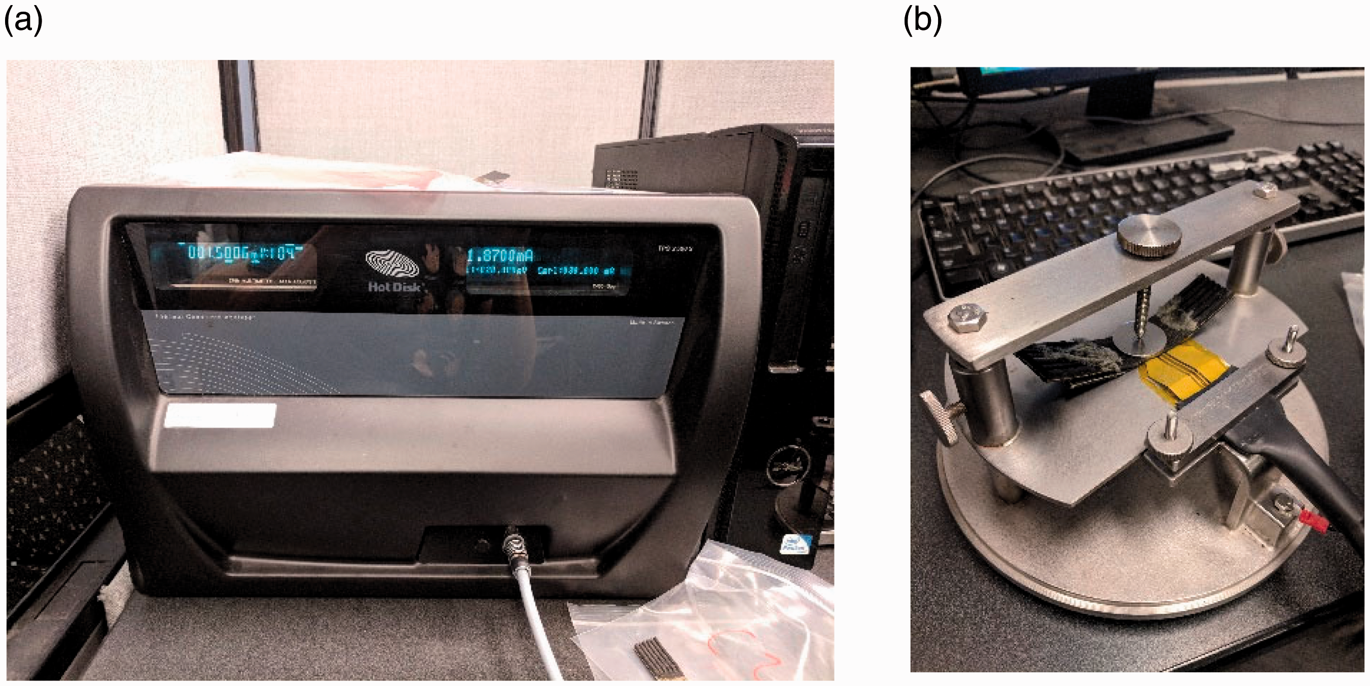
(a) Hot Disk TPS 2500S and (b) measurement of thermal conductivity.

Second, the heat transfer coefficient h_p is measured through an experiment. It is primarily related to the local air velocity V_p and material properties. In this application, the relationship between h_p and the local air velocity is shown as the solid line in Figure 11. This study uses equation (10) to fit the curve (dashed line in Figure 11) to the experimental data, and the three coefficients for equation (10) are measured as k_h = −0.0053, p_h = 1.1, and q_h = 14.

Figure 11.

Relationship between h_p and V_p.

Experiment

A five-pulley-belt drive system was also designed (see Figure 12(a)) and installed on an engine test system (see Figure 12(b)). In this belt system, there were two primary pulleys: the DR pulley marked as Pulley 1 and the DN pulley marked as Pulley 4. The other three were auxiliary pulleys. Pulley 2 was mounted on a hub load sensor for belt tension measurement. Pulley 3 was mounted on a speedometer for belt speed measurement. Pulley 5 was mounted on a tensioner to reduce the vibration of the belt and keep the belt tension constant. The temperature of the environment is also critical, so a customized insulated chamber was mounted on the engine simulator, enclosing the belt drive system. Two thermocouples on the two sides of the chamber monitored the inside temperature. A case fan inside this chamber ensured that the chamber temperature was uniformly distributed. Furthermore, a thermal graphic camera was installed to target the DN pulley and measure its temperature distribution during the test.

Figure 12.

(a) Belt layout and (b) installation of the experimental belt system.

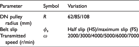
To validate the accuracy of the thermal model for various pulley sizes under a number of operating conditions, this experiment examined several factors (see Table 2) that influence the temperature distribution of a pulley. The first factor was the pulley radius. Radii of 62 and 108 mm are the minimum and maximum sizes of industrial pulleys. A midrange pulley with a radius of 85 mm was also selected. The second factor was the belt slip, which is caused by transmitted torque. However, it is impractical to use belt slip to investigate the influence of torque on the temperature distribution of a pulley because of the significant variation in pulley radii considered as the first factor. The third factor was the rotation speed, which ranged from 2000 to 7000 r/min, representing a dramatic change in the engine operating conditions.

Table 2.

Operating parameters.

Parameter	Symbol	Variation
DN pulley radius (mm)	R	62/85/108
Belt slip	ϕ_s	Half slip (HS)/maximum slip (FS)
Transmitted speed (r/min)	ω	2000/3000/4000/5000/6000/7000

The thermal model used the above information related to the belt layout and operating conditions, together with the pulley geometries and thermal properties (h, λ_p, …) measured based on standard procedures, to calculate the temperature distributions of the DN pulley under the designated operating conditions.

Results and discussion

To demonstrate the accuracy of this model, this work exhibits validation through comparing the analytical temperatures at the outer radius of pulley with the experimental values under the various pulley radii, belt slip types, and speeds listed in Table 2. Temperatures at this location are critical for determining thermal failures of materials, because the temperature at the outer radius is the highest temperature in the pulley.

At the beginning of operation, the radius of a pulley influences the temperature distribution. First, large pulleys present more dissipation surface area to the environment than do small pulleys. Second, the heat transfer coefficient at the edge of a large pulley is higher than that of a small pulley because large pulleys have higher tangential speeds. Pulleys with large radii therefore have lower temperatures than pulleys with small radii. Figure 13 shows the analytical temperatures at the outer radii of three pulleys with different radii under the condition of 3000-r/min rotation and the half-slip rate. The decrease in the temperature with an increase in the radius predicts the trend described above. These results are in good agreement with the experimental data.

Figure 13.

Comparisons of analytical and experimental temperatures at the outer radii of three pulleys at a rotational speed of 3000 r/min and the half-slip operating condition.

Increased belt slip leads to higher thermal generation and higher peak temperatures on the outside radius of the pulley. In this experiment, different torque loads were applied to DN pulleys to achieve different slip rates. Figure 14(a) and (b) presents the analytical temperatures at the outside radii of two pulleys under the conditions of half and maximum slip. The results showed the same tendencies as those observed in the measurements.

Figure 14.

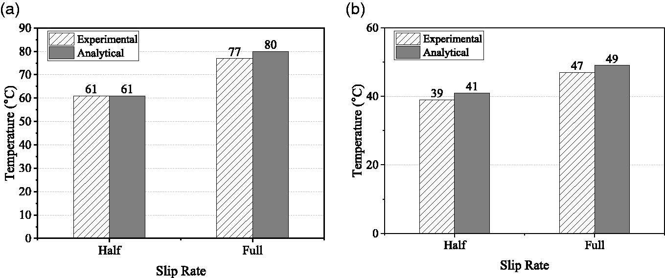
Comparisons of the analytical and experimental temperatures at the outer radii of two pulleys at a rotational speed of 2000 r/min and the half and maximum slip operating condition, set at (a) 62-mm pulley and (b) 108-mm pulley.

Another factor in evaluating the accuracy of a thermal model was a comparison of the analytical and experimental temperatures under different transmitted speeds. Unlike torque changes, shifts in speed alter not only thermal generation but also heat dissipation on surfaces. Figure 15 exhibits the analytical temperatures at the outside radius of a 108-mm pulley under half-slip conditions. The temperature on the outside radii of the pulley increased in response to the increase in speed. The results demonstrate that the rise in heat generation is more significant than the effect of the heat transfer coefficients. The consistency between the experimental and analytical temperatures shown in Figure 15 shows that the thermal model can accurately capture this trend of temperature rise.

Figure 15.

Temperature comparisons for the 108-mm pulley at various speeds under half-slip conditions.

The temperature distribution of a pulley is also critical because the accuracy of this measurement ensures that the thermal model will calculate the pulley’s precise heat dissipation and λ_p. Figure 16 shows four points along the pulley’s radial direction that validate the pulley’s temperature distribution. Figure 17 shows comparisons of the temperature distributions of two pulleys under various conditions. The model successfully predicted the temperature decrease from the outer to the inner radial distances. The analytical temperature plots are in good agreement with the measurement data.

Figure 16.

Selected points along the pulley radius.

Figure 17.

Experimental versus analytical temperature distributions at P1–P4 for (a) a 62-mm pulley at two slip rates and (b) a 108-mm pulley at two rotational speeds.

Some notable differences remain between the prediction and experiment. One reason for these differences is measurement error, which is impossible to eliminate completely. The second reason is that equation (4) is a curve-fitting equation, which provides an approximate value of h for this thermal analysis. Nevertheless, the above figures generally show good agreement between the predicted and experimental values.

Most importantly, all the above predictions provided by the thermal model require much less computational time and resources than do the numerical approaches. The pulley temperature prediction for a five-pulley-belt drive system requires less than 5 s on a desktop with a 16-core 3.4-GHz AMD CPU and 32-GB memory, while the current numerical method requires approximately 17 h³³ for the temperature prediction of a belt drive system. In summary, the above temperature comparison demonstrates that this thermal model can provide reliable and time-efficient temperature predictions.

Conclusion

This study presents a novel pulley thermal model to enable pulley temperature distribution prediction in an accurate and efficient manner. Because the existing analytical research is not suitable for pulley irregular structures and because the computational time of numerical approaches under abundant belt drive load cases is beyond the feasible dimension, a thermal model that achieves quick and precise temperature calculation is necessary. The main challenge and innovation of this research is creating an analytical model that takes into account the comprehensive pulley structure to achieve accurate pulley temperature prediction. The analytical algorithm in this model also guarantees the quick delivery of temperature results, reducing the calculation time from 17 h³³ to less than 5 s for each static operation condition. In addition, variables are used to represent the pulley dimensions. As a result, the model can be implemented in a relatively simple manner for any pulley size. A polynomial is adopted to represent the relationship between the local speed and thermal dissipation coefficient, making this model applicable for various materials and their heat dissipation situations. A comparison of the experimental and analytical results at various selected locations under various operating conditions demonstrates the accuracy of the model. In summary, the time-efficient and accurate pulley model can be used to predict temperatures for high-temperature resistance material selection in the early design stages. Moreover, the presented model is beneficial for predicting temperatures under a variety of engine load cases for subsequent material fatigue analysis. Furthermore, this thermal model has considerable potential for use in the belt drive industry.

Footnotes

Handling Editor: James Baldwin

Declaration of conflicting interests

The author(s) declared no potential conflicts of interest with respect to the research, authorship, and/or publication of this article.

Funding

The author(s) disclosed receipt of the following financial support for the research, authorship, and/or publication of this article: Funding for this research from Mitacs Canada and the Litens Automotive Group is gratefully acknowledged.

ORCID iD

Xingchen Liu

References

Caputo

Millo

Boccardo

, et al. Numerical and experimental investigation of a piston thermal barrier coating for an automotive diesel engine application. Appl Therm Eng 2019; 162: 114233.

Gerbert

Traction belt mechanics. Göteborg: Machine and Vehicle Design, Chalmers University of Technology, 1999.

Manin

Liang

Lorenzon

Power losses prediction in poly-v belt transmissions: application to front engine accessory drives. In: International gear conference, Lyon, 26–28 August 2014, pp.1162–1171. New York: Elsevier.

Bertini

Carmignani

Frendo

Analytical model for the power losses in rubber V-belt continuously variable transmission (CVT). Mech Mach Theory 2014; 78: 289–306.

Silva

CAF

Manin

Rinaldi

, et al. Modeling of power losses in poly-V belt transmissions: hysteresis phenomena (standard analysis). J Adv Mech Des Syst Manuf 2017; 11: JAMDSM0085.

Silva

CAF

Manin

Rinaldi

, et al. Modeling of power losses in poly-V belt transmissions: hysteresis phenomena (enhanced analysis). Mech Mach Theory 2018; 121: 373–397.

Silva

Manin

Andrianoely

M-A

, et al. Power losses distribution in serpentine belt drive: Modelling and experiments. Proc IMechE, Part D: J Automobile Engineering 2019; 233: 3424–3437.

Balta

Sonmez

Cengiz

Speed losses in V-ribbed belt drives. Mech Mach Theory 2015; 86: 1–14.

Qin

Cui

Yan

, et al. Hysteresis modeling of clamp band joint with macro-slip. Mech Syst Signal Process 2016; 66–67: 89–110.

10.

Julió

Plante

JS.

An experimentally-validated model of rubber-belt CVT mechanics. Mech Mach Theory 2011; 46: 1037–1053.

11.

Goswami

Sardar

Karmakar

SK.

Temperature rise and wear of sliding contact of alloy steels. AIP Conf Proc 2016; 1754: 030004.

12.

Hou

Komanduri

General solutions for stationary/moving plane heat source problems in manufacturing and tribology. Int J Heat Mass Transf 2000; 43: 1679–1698.

13.

Komanduri

Hou

ZB.

Analysis of heat partition and temperature distribution in sliding systems. Wear 2001; 251: 925–938.

14.

Laraqi

Alilat

de Maria

JMG

, et al. Temperature and division of heat in a pin-on-disc frictional device—Exact analytical solution. Wear 2009; 266: 765–770.

15.

Yevtushenko

Kuciej

Och

Modeling of the temperature regime and stress state in the thermal sensitive pad-disk brake system. Adv Mech Eng 2018; 10: 1–12.

16.

Vick

Furey

MJ.

A basic theoretical study of the temperature rise in sliding contact with multiple contacts. Tribol Int 2001; 34: 823–829.

17.

Zhang

Yin

Liu

, et al. Thermal–structural coupling analysis of brake friction pair based on the displacement gradient circulation method. Adv Mech Eng 2018; 10: 1–13.

18.

Waddad

Magnier

Dufrénoy

, et al. Heat partition and surface temperature in sliding contact systems of rough surfaces. Int J Heat Mass Transf 2019; 137: 1167–1182.

19.

Coulibaly

Chassaing

Philippon

Thermomechanical coupling of rough contact asperities sliding at very high velocity. Tribol Int 2014; 77: 86–96.

20.

Nosko

Partition of friction heat between sliding semispaces due to adhesion-deformational heat generation. Int J Heat Mass Transf 2013; 64: 1189–1195.

21.

Talati

Jalalifar

Analysis of heat conduction in a disk brake system. Heat Mass Transf 2009; 45: 1047–1059.

22.

Phan

Kondyles

Rotor design and analysis; a technique using computational fluid dynamics (CFD) and heat transfer analysis. SAE technical paper 2003-01-3303, 2003.

23.

Reddy

Mallikarjuna

Ganesan

Flow and heat transfer analysis of a ventilated disc brake rotor using CFD. SAE technical paper 2008-01-0822, 2008.

24.

Yan

Feng

Yang

, et al. Role of cross-drilled holes in enhanced cooling of ventilated brake discs. Appl Therm Eng 2015; 91: 318–333.

25.

Moradi-Dastjerdi

Payganeh

Tajdari

Thermoelastic analysis of functionally graded cylinders reinforced by wavy CNT using a mesh-free method. Polym Compos 2018; 39: 2190–2201.

26.

Moradi-Dastjerdi

Behdinan

Thermoelastic static and vibrational behaviors of nanocomposite thick cylinders reinforced with graphene. Steel Compos Struct 2019; 31: 529–539.

27.

Safaei

Moradi-Dastjerdi

Qin

, et al. Determination of thermoelastic stress wave propagation in nanocomposite sandwich plates reinforced by clusters of carbon nanotubes. J Sandw Struct Mater. Epub ahead of print 8 May 2019. DOI: 10.1177/1099636219848282.

28.

Belhocine

Bouchetara

Thermal behavior of full and ventilated disc brakes of vehicles. J Mech Sci Technol 2012; 26: 3643–3652.

29.

Nasif

Barron

Balachandar

Simulation of jet impingement heat transfer onto a moving disc. Int J Heat Mass Transf 2015; 80: 539–550.

30.

Pellé

Harmand

Heat transfer study in a rotor–stator system air-gap with an axial inflow. Appl Therm Eng 2009; 29: 1532–1543.

31.

Lallave

Rahman

Kumar

Numerical analysis of heat transfer on a rotating disk surface under confined liquid jet impingement. Int J Heat Fluid Flow 2007; 28: 720–734.

32.

Lallave

Rahman

MM.

Numerical simulation of transient thermal transport on a rotating disk under partially confined laminar liquid jet impingement. J Heat Transfer 2010; 132: 052201.

33.

Wurm

Fitl

Gumpesberger

, et al. Novel CFD approach for the thermal analysis of a continuous variable transmission (CVT). Appl Therm Eng 2016; 103: 159–169.

34.

Wurm

Fitl

Gumpesberger

, et al. Advanced heat transfer analysis of continuously variable transmissions (CVT). Appl Therm Eng 2017; 114: 545–553.

35.

Wei

Kan

Zhang

, et al. The frictional energy dissipation and interfacial heat conduction in the sliding interface. AIP Adv 2018; 8: 115321.

36.

Bhushan

Modern tribology handbook. Boca Raton, FL: CRC Press, 2001.

37.

Shiming

Wenquan

Heat transfer. 4th ed. vol. 1. Beijing, China: Higher Education Press, 1998.

38.

Komen

EMJ

Frederix

EMA

Coppen

THJ

, et al. Analysis of the numerical dissipation rate of different Runge–Kutta and velocity interpolation methods in an unstructured collocated finite volume method in OpenFOAM®. Comput Phys Commun. Epub ahead of print 20 January 2020. DOI: 10.1016/j.cpc.2020.107145.

39.

Ishkhanyan

AM.

Solutions of the bi-confluent Heun equation in terms of the Hermite functions. Ann Phys 2017; 383: 79–91.

A novel analytical model for the thermal behavior of a fiber-reinforced plastic pulley in a front-end accessory drive

Abstract

Keywords

Introduction

Pulley thermal analytical model

Overall calculation process

Determining the heat source information in the pulley system

Determining the heat partition coefficient

Pulley internal thermal analysis

Measurement of input parameters

Experiment

Results and discussion

Conclusion

Footnotes

Declaration of conflicting interests

Funding

ORCID iD

References