
Abstract
The difficulty of knowing the real-time status of gas face seals is the main cause of common problems, including sudden failure, ineffective diagnosis, and unpredictability of service life. This study analyzed the acoustic emission signals generated from experiments, uncovering their features in terms of the frequency distribution, periodic fluctuations, and the behaviors during different operation phases. A new vectorization procedure was designed according to the knowledge of informative acoustic emission features. Based on the vectorization procedure, a support vector machine regression method was applied to develop models predicting the eccentric load on the stator of the seal. Cross-validation was conducted to evaluate the regression performance and search for a proper kernel scale. This study found the informative features of acoustic emissions at different timescales and during different seal operation phases, and particularly the great informative potential of certain segments of the starting and stopping phases. The vectorization and support vector machine regression were shown to be effective in estimating the loads in experiments with cross-validation. Thus, a method for estimating the status of gas face seals based on acoustic emission monitoring was established.
Introduction
The mechanical face seal is a commonly used type of shaft end seal. As a kind of noncontacting mechanical face seal, the gas face seal is intended to work with faces that are totally separated by gas. This expands their service life even under high pressure and/or speed conditions, and is the main reason for their widespread use. However, mechanical face seals frequently suffer from problems, including sudden failure, ineffective diagnosis, and unpredictability of service life.1,2 This is mainly attributed to the difficulty of determining the status of seals with online measured signals.
Besides measuring the flow rate, pressure, and temperature of the fluid leaked as a basic performance evaluation, efforts have been made in order to get detailed information. 2 Among them, acoustic emission (AE) monitoring, which is traditionally applied to the identification of material defects, 3 is considered as a monitoring method with high potential, owing to its outstanding information density, 2 friction sensitivity, and engineering practicability. In the 1990s, Miettinen and Siekkinen 4 and Holenstein 5 reported early success in detecting tribological behaviors, including friction and leakage, with well-positioned sensors. Braccesi and Valigi 6 investigated the periodic fluctuation of the AEs and torque of a noncontacting mechanical face seal. Towsyfyan et al. 7 analyzed the AE features, including RMS (root mean square) and kurtosis under different lubrication regimes, in a mechanical seal. He also studied the AE features related to some common failures. 8 In previous studies, 9 we investigated AEs generated by a gas face seal, and validated that AEs contain abundant information, allowing for a certain degree of interpretation. However, it is difficult to develop a physical-mechanism-based model that can comprehensively consider various factors to determine the status of seals according to the AEs obtained.
An alternative solution is to apply machine learning methods to develop a predictive model based on empirical data. This only requires some incomplete knowledge with regard to the physical mechanisms, based on which an extraction for the informative AE features can be performed. A few studies have attempted to apply machine learning to the AE signals generated from mechanical seals. Zhang and Li 10 developed artificial neural networks (ANNs) which distinguished between the intervals wherein the seal face separation lies using AE signals decomposed with wavelet transform. Li et al. 11 developed a method based on the genetic particle filters with autoregression and hypersphere support vector machines (SVMs) to distinguish between the contact state categories using AE signals. Xiao et al. 12 developed an ANN model to estimate film thickness based on AE signals processed with wavelet analysis and kernel principal component analysis.
The existing research of employing AE signals to estimate seal status used kinds of parameters which represent the overall properties of the AEs in a considerable duration of running as the predictors to establish machine learning models. The work being presented is intended to raise a different approach in feature engineering for gas face seal AEs, which focuses on exploiting features at different timescales and during the different operation phases of the seal.
In the work being presented, the AEs generated from experiments on a gas face seal test rig were first studied in terms of their frequency distribution, periodic fluctuations, and the behaviors during different operation phases. The AEs were vectorized according to the knowledge of their features. Based on the vectorized AE data, the models were developed using SVM regression to predict the targeted parameter, and tested using a particular cross-validation policy. In summary, a method of estimating the status of a gas face seal was developed and validated.
AEs and their informative features
Acquiring AE signals through experiments
Experiments were previously performed 9 with a test rig as shown in Figure 1. The rig employed two spiral groove gas seals sharing one rigidly mounted rotating ring, namely rotor, with spiral grooves (Figure 2) on both faces. The grooves were intended to keep the two flexibly mounted non-rotating rings, namely stators, from making contact with the rotor, by providing a hydrodynamic effect (which is weak during starting/stopping) and a hydrostatic effect.

Illustration of the test rig: loading mechanism and AE sensor appended to gas face seal.

Spiral grooves on rotor.
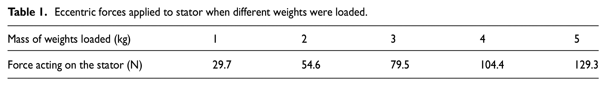
A loading mechanism was appended to the outer stator to push and tilt the stator, and thus induce contact. The eccentric forces applied when different weight masses were loaded are listed in Table 1. A miniature acoustic emission sensor (model PICO by Physical Acoustic Corporation), as shown in Figure 3, was mounted onto the back of the outer stator with a penetration assembly to record one AE wave every 1.3 ms. Each wave contained
Eccentric forces applied to stator when different weights were loaded.

The PICO AE sensor employed.
In this study, we used the results of 10 of the experiments with the fixed speed of 1200 r/min, gauge pressure of 4 atm, and the varying rotor tilt and load (represented by the mass of loaded weights) as presented in Table 2.
Operating conditions.

Mass of loaded weights.
Informative features of AEs generated by gas face seal
In this section, we are going to take a careful analysis on the AEs to study how are the AE waves different from each other and how do the differences relate to the status of the gas face seal. They are beneficial for investigating gas face seal AEs effectively, and are also the basis of vectorization, which is an essential step toward establishing machine learning model to estimate the seal’s status.
AE features at different timescales
Let us consider the experiment with the 46-µrad rotor tilt and 3-kg load as an example. The frequency spectrums of a few AE waves, which are illustrated in Figure 4, imply that the AE power is concentrated on several fixed bands. The frequency distribution of the AE waves at different times had different modes. As can be seen in Figure 4(b2) and (b3), the AE power tended to concentrate in the proximity of 490 kHz at

Frequency distributions in experiment with the 46-µrad rotor tilt and 3-kg load, and dynamic fluctuation of AE RMS.
Because AE monitoring typically has a high sample rate, the features of every individual AE wave (typically the above-mentioned frequency distribution) and the fluctuations with dynamic excitation appeared at distinguishable timescales, which contain their respective information. To consider both timescales, band filters were applied at 170 ± 40 kHz, 280 ± 40 kHz, and 490 ± 40 kHz. Then, the time series of RMS before filtering and after filtering (with three different filters) could represent the dynamic fluctuations of AEs, as shown in Figure 5, by considering the experiment with the 46-µrad rotor tilt and 2-kg load as an example.

Phases in gas seal operation for experiment with 46-µrad rotor tilt and 2-kg load; starting phase I, starting phase II, stable operation phase, stopping phase II, and stopping phase I proceeded in sequence.
AE features by operation phases
As marked in Figure 5, different features were observed in the sequential phases of the entire process, as follows:
Starting phase I: Within 1 s after starting, the RMS first increased to a high level of
Starting phase II: After the starting phase I, that is, after the RMS decreased to a normal level, the AEs fluctuated periodically. Moreover, such periodic fluctuations changed as the speed increased. In the rest of this article, this phenomenon will be referred to as quasi-periodicity.
Stable operation phase: The speed eventually stabilized at 1200 r/min. Then, the AEs kept exhibiting periodic patterns.
Stopping phase II: As the seal began to shut down, the AEs remained periodic within any short duration and changed as the speed decreased. This demonstrates the above-mentioned quasi-periodicity in the same manner as during the starting phase II, but reversed.
Stopping phase I: Within 1 s before a complete stop, the AEs increased and decreased in a similar manner as during the starting phase I, but reversed.
To estimate the seal status from the AEs, we had to determine whether the major discrepancies exhibited by the AEs could be attributed to the controlled differences rather than to the other factors. This was investigated with different phases, respectively, as follows:
1. Stable operation phase
Figure 6 shows the original and filtered RMS during the stable operation phase for all 10 experiments. Like the mentioned examples, good periodicity was observed. As the load increased, the AE fluctuations sequentially exhibited calm, intermittent, and full-period features. 9 The RMS ratio between the AEs processed with the three band filters, respectively, did not keep constant; that is, the frequency distribution exhibited discrepant modes, as above-mentioned.

Stable operation phase. With a light load, the AE signals were calm. As the load increased, the signals exhibited intermittent features and eventually became full-period.
Because the signals could be weak (with RMS below 10 mV) when a light load was exerted, it was estimated that the noise was even weaker than that. Hence, there was no need for denoising. This advantage was attributed to the direct mounting of the AE sensor onto the stator.
2. Starting phase I and stopping phase I
The starting phase I and stopping phase I possessed very similar features; therefore, they will be discussed together. As can be seen in Figure 7, unlike the stable operation phase, regularity was not observed with the change of the operating conditions, which means the AEs in these phases were sensitive to other uncontrolled random factors, rather than to the variation of the load and rotor tilt. Thus, they were excluded because they were not suitable for estimating the status of the seal.
3. Starting phase II and stopping phase II
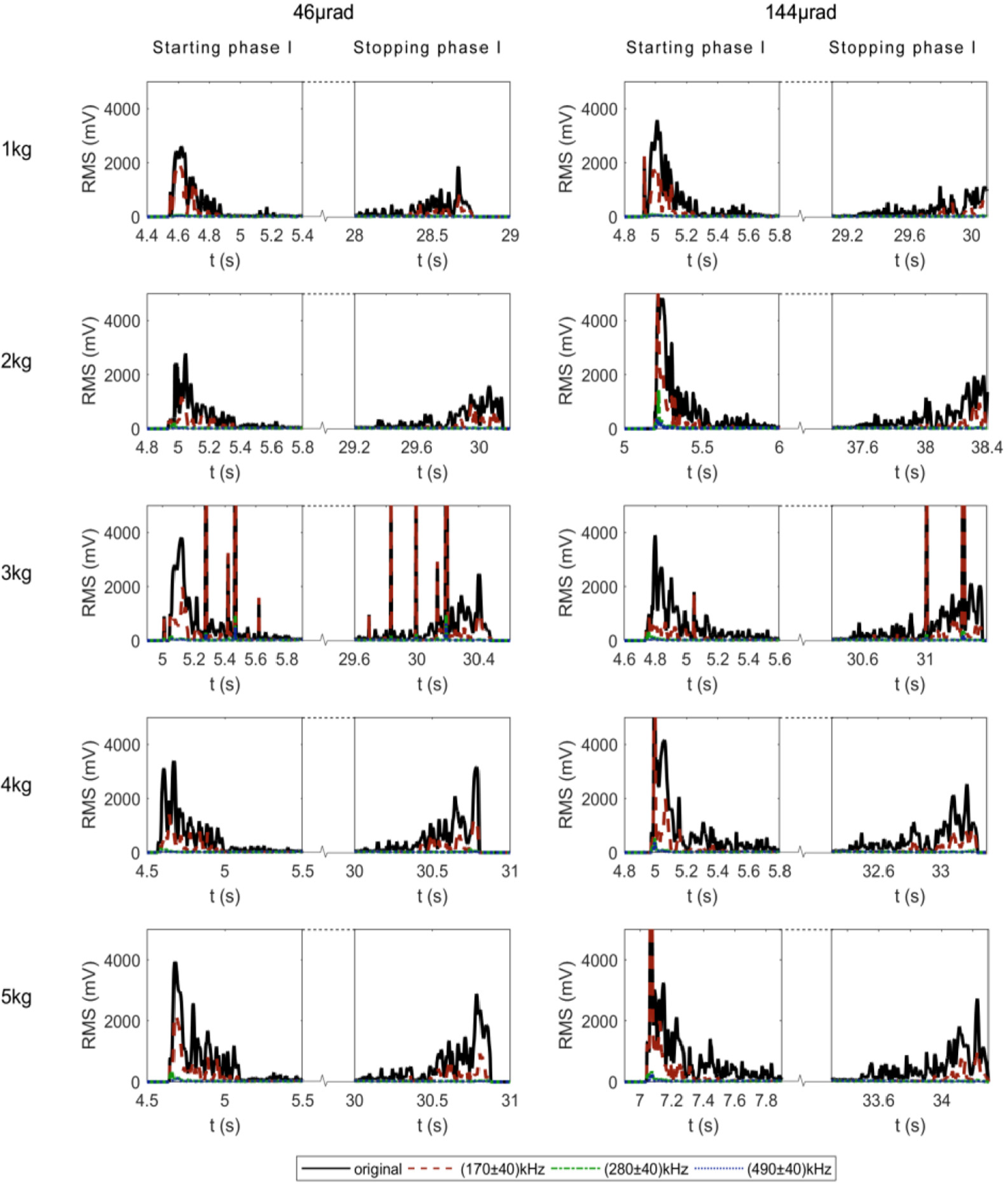
Starting phase I and stopping phase I. The AE signals were irregular and thus unsuitable for estimating the status of the seal.
The regular AE changes with the operating conditions during the starting phase II and the stopping phase II, as shown in Figure 8, were similar to those during the stable operation phase. Unlike the stable operation phase, during which the signals repeated themselves with a constant period, the quasi-periodic signals possessed more informative content as they varied with speed.

Staring phase II and stopping phase II. Although the AE signals changed with speed, they still appeared as periodic within any short duration and thus exhibited quasi-periodicity.
A summary on the AE features
In summary, the following features are found from the AEs generated by the gas face seal:
Regarding the timescale of individual AE waves, or at an acoustic timescale, the power was concentrated in several fixed frequency bands with discrepant modes. This means that the RMS of each AE wave processed with corresponding band filters can carry the major information of the frequency distribution.
The dynamic behaviors of the seal were reflected by the RMS fluctuations of the AEs processed by different band filters or by the features at a dynamic timescale.
During the stable operation phase, the AEs exhibited periodicity that was synchronous with the shaft; during the starting/stopping phase II, they exhibited quasi-periodicity. Both of these phenomena developed regularly as the operating conditions changed, unlike the starting/stopping phase I, which did not exhibit the above-mentioned regularity.
The knowledge of informative AE features will be a basis for vectorizing them during establishing machine learning model, which will be discussed in the “Vectorization of AE signals” section.
Estimating seal status using SVM regression
To estimate the status of seal, steps including preparing the dataset, employing a machine learning model, training it, and validating the estimation performance were needed. The dataset came from the experiment described in the “Acquiring AE signals through experiments” section and was converted into feature vectors according to the knowledge of informative features concluded in the “Informative features of AEs generated by gas face seal” section. Figure 9 gives an overview of the steps.

An overview of the steps to estimate the status of the gas face seal.
SVM regression
A model that maps a vector representing the AE features to a parameter dominating the seal’s status should be established in order to make an estimation. Here, the eccentric load on the stator was targeted. The experiments provided AE data with known loads. The development of a model based on such data belongs to the supervised learning.
Supervised learning, including classification and regression, can be briefly described as learning from known empirical data, in the form of
The idea of SVMs was introduced by Vapnik 14 in 1992. In regression problems, this method searches for a hyperplane whose deviation from the training data is as little as possible. 13 The SVM method performs well even with a small sample. With suitable kernels, the SVM method is capable of handling nonlinear problems.
Let us assume that

Here,

The optimized hyperplane is searched by minimizing

under the following constraints


The optimization is solved using the Lagrangian multiplier method, calculated using sequential minimal optimization (SMO) algorithm, yielding
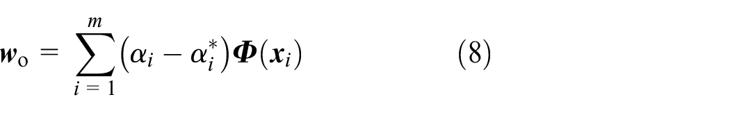
Here,
The approximated function is expressed as follows

Let us define the kernel function as
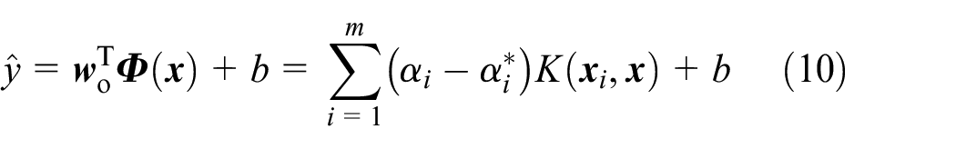
An explicit

Here,
Vectorization of AE signals
As has already been mentioned, when using SVM (or most of the other supervised learning methods), the empirical data must be represented by vectors as
The vectorization procedure was designed based on the conclusions, that is, the knowledge about the informative features of AEs, presented in the “Informative features of AEs generated by gas face seal” section. An initial idea is to divide the AEs into a large number of segments and turn each segment into a vector. Because of the repetition of the AEs during the stable operation phase, it is not effective to adopt the entire stable operation phase because a few periods are sufficient. Conversely, the quasi-periodic starting phase II and stopping phase II can contribute a great number of distinct vectors, and thus are the major data source for estimating the status of the seal. However, there exists another problem whereby the count of AE waves in each period changes with the speed during the starting/stopping phase II, although the representing vector should have fixed dimensionality. Therefore, the AEs were vectorized as follows:
Two paragraphs, namely, the starting phase II along with the conterminous beginning (a few periods) of the stable operation phase, and the stopping phase II along with the conterminous ending of the stable operation phase, were taken from each experiment.
For each paragraph, a new series of moments was determined by setting 30 moments in each instantaneous rotary shaft period. Three band power indices (corresponding to the three key bands) were interpolated at each moment by applying the locally weighted average (employing a fine Gaussian kernel) to the RMS of the band filtered waves and then dividing by the average RMS of the entire paragraph to rule out the effect of the overall RMS scale. Three series of band power indices,
Every consecutive nT term


Here,

Vectorization of AE signals for experiment with 46-µrad rotor tilt and 3-kg load.
In the procedure outlined above, a large number of predictors, with 90 features, were generated from the 10 experiments, or 20 AE paragraphs, as presented in Table 3.
Count of generated observations.
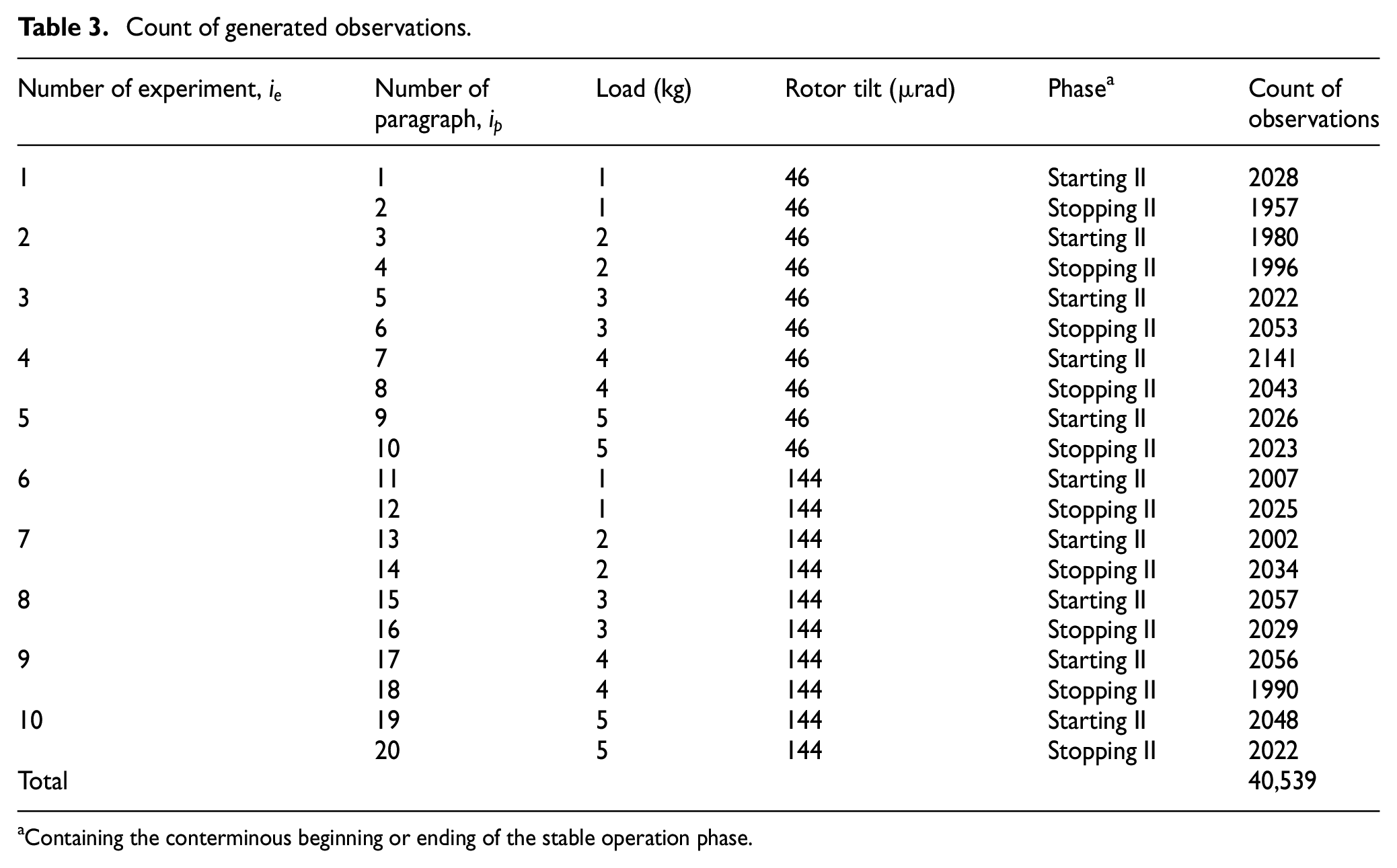
Containing the conterminous beginning or ending of the stable operation phase.
As mentioned in the “SVM regression” section, the role of the response, or parameter to be predicted by the regression, was played by the load (mass of loaded weights, in kilograms), which is a quantitative parameter.
Validation results and discussion
The SVM regression models were ready to be developed based on the vectorized predictors and responses, which were generated as described above. To evaluate the performance of the models developed using the proposed method, cross-validation was necessary, because testing the performance using the data contained in the training set may dramatically underestimate the error.
The commonly used k-fold validation could have been easily implemented. However, to evaluate the model’s performance for a new experiment, instead of a new observation, a stricter policy was used: each of the 10 experiments was ruled out and the model was trained using the observations generated from the other 9 experiments. Then, the model was tested using the observations generated from the excluded experiment. In other words, it was assumed that the load for the nine experiments was known, while the load of the excluded experiment was to be determined. Hereafter, this will be referred to as a “leave-one-experiment-out” cross-validation.
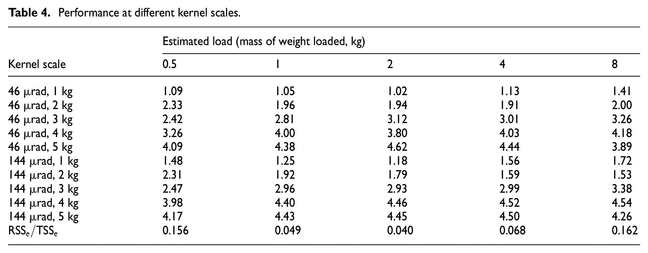
After obtaining the predicted responses of the observations generated from the excluded experiment, the average value of the responses was considered as its estimated load. Table 4 and Figure 11 present the estimated load along with the performance evaluation with different kernel scales. The residual sum of squares (RSS) at the level of the experiments, which is defined below, was calculated and normalized by dividing it with the total sum of squares (TSS) to quantify the error when estimating the load


Performance at different kernel scales.

Cross-validation results at different kernel scales: (a)–(e) estimated load and (f) comparison of
The following conclusions were drawn from the cross-validation results:
When the kernel scale was 1, 2, or 4, the method performed well
The loads for the two experiments with the 5-kg load were underestimated, whereas the loads for the two experiments with the 1-kg load were overestimated. This means that the proposed method performed better when disregarding the edges of the data.
Conclusion
The AEs generated from experiments on a gas face seal test rig under different operating conditions were analyzed. An AE vectorization procedure was designed based on the knowledge of informative AE features. A cross-validation policy was used to evaluate the SVM regression performance for an experiment excluded from the training set, and to search for a proper kernel scale.
The conclusions drawn from this study are as follows:
From a cross-timescale perspective, it was revealed that the AEs exhibited different features with regard to the different physical mechanisms. At the timescale of individual AE waves, or acoustic timescale, the AE power concentrated in several fixed bands with discrepant modes. At the timescale of fluctuations with dynamic shaft perturbation, or dynamic timescale, the AEs had good periodicity during the stable operation phase, and quasi-periodicity during part of the starting phase (except for the very beginning) and part of the stopping phase (except for the very ending). In addition, they developed regularly with the changes of the operating conditions in these durations.
Based on the knowledge of informative AE features, the AE power concentration in several key bands within certain durations, mainly the quasi-periodicity parts of the starting and stopping phases, was used to generate the representative vectors. A “leave-one-experiment-out” cross-validation was conducted for the SVM regression models. The validation demonstrated that the load of the experiment excluded from the training set could be adequately estimated, and provided an approach toward finding the proper hyper-parameter.
This article proposes a method of estimating the status of gas face seals by applying machine learning techniques based on measurable signals, which are vectorized according to the knowledge of their informative features. The study can be useful as a reference for monitoring other types of equipment. Moreover, the success of using the data from the starting and stopping phases implies that the nonsteady process can be valuable in diagnosis.
Footnotes
Handling Editor: James Baldwin
Declaration of conflicting interests
The author(s) declared no potential conflicts of interest with respect to the research, authorship, and/or publication of this article.
Funding
The author(s) disclosed receipt of the following financial support for the research, authorship, and/or publication of this article: This study was supported by the National Key Research and Development Program of China (Grant No. 2018YFB2000800) and the National Natural Science Foundation of China (Grant Nos U1737209 and 51735006).