Extended singular robust inverse solution of redundant serial manipulators

Abstract

We propose the use of a damping matrix β to replace the unified damping coefficient λ in the singular robust inverse method, allowing for adjustment of the manipulator’s singularity for different joints separately. In addition, the correction coefficient matrix α is employed to eliminate the Jacobian matrix approximation error, which usually exists in the iterative control solving process; the extended singular robust inverse method is thereby proposed. This article contains analyses of the singularities caused by three methods and how they result in larger values of the manipulator terminal error and joint angular velocity; additionally, the semi-empirical selection principles of β and α are given. The stability of the proposed method is investigated with the Lyapunov stability criteria, and its effectiveness is verified for spatial linear and curve trajectories with 7-axis and 10-axis redundant serial manipulators. The simulation results show that the proposed method exhibits improved optimization performance and stability, and the terminal error is stable and within the allowable range. The least singular value is larger and the joint angular velocity is the lowest, which is the expected outcome. Furthermore, the simulation results for the 10-axis manipulator also indicate the generality of the proposed method.

Introduction

Kinematics control is one of the most general issues in robot manipulator technology, in which the focus is on the inverse kinematics solution.^1–8 However, it is often difficult to find a suitable solution for redundant manipulators due to high nonlinearity. There have been many studies on classical methods used to find the pseudoinverse solution of various target functions.^2,3,6,9–13

The singular value decomposition generalized inverse method (SGIM) is a typical and widely used method for solving inverse motion of redundant manipulators, and it provides a defined Jacobian generalized inverse by singular value decomposition.^8,10,14,15 The optimization object of SGIM is the least squares solution with the minimum norm.^10,15 However, when the minimum singular value approaches 0, the norm of angular velocity tends to infinity, and the resulting solution has no practical significance for the control operation.

Therefore, another new scheme, the singular robust inverse method (SRIM), has been proposed and widely used in inverse kinematics of redundant manipulators.^{11–13,16–22} Unlike SGIM, SRIM introduces the damping coefficient λ to avoid problems caused by small singular values and reconstructs a new optimization target function. However, the optimization effect is largely decided by the selection of the damping factor λ and, in recent years, scholars have proposed various definitions of λ. Wampler suggested that λ was a constant. ¹¹ Nakamura and Hanafusa, ¹⁷ Kelmar and Khosla, ¹⁸ Chan and Lawrence, ¹⁹ and others^13,20 have proposed a definition of the piecewise function of λ. In addition, intelligent algorithms have also been used in recent years to find better damping factor values. ²¹

Compared with SGIM, SRIM has achieved better results in solving the inverse motion of trajectory tracking, but there also exist some shortcomings. They are as follows:

1. A uniform value of damping factor λ is usually employed in SRIM solutions without considering the optimization requirements of each singular value. As a result, the over-optimization of large singular values results in redundant errors and singularities.

2. In order to effect the change of joint angle Δθ from t_k to t_k+1 during the iteration process, the Jacobian matrix is usually considered unchanged and the Jacobian matrix at t_k is considered an approximation substitution value. Once the manipulator passes a singular point between t_k and t_k+1, the singular values of the Jacobian matrix will change significantly and the approximation will produce a larger terminal error. The error can be eliminated by employing a smaller sampling interval, but more computing resource will then be consumed. Obviously, neither SRIM nor SGIM considers the effect of the approximation.

To eliminate the defects of SRIM, we propose to introduce the damping matrix β instead of the unified damping factor λ. A pre-factor matrix α is also employed to eliminate the error caused by approximation of the Jacobian matrix and the extended singular robust inverse method (ESRIM) results. Subsequently, a comparative analysis and simulation examples show that using the proposed method, the stability of the ESRIM is significantly improved and results in the desired end error, smaller joint angular velocity, and larger least singular value.

This article introduces the modified coefficient matrices to overcome the shortcomings of the SRIM. An introduction to the SGIM and SRIM models is shown in section “Preliminaries” and the new methodology ESRIM is illustrated in section “New singularity-avoidance scheme.” In section “Simulation analysis verification,” the modified method is applied to a 7-axis manipulator and a 10-axis manipulator, respectively, for validation and comparison. Section “Conclusion” presents the conclusions drawn from this work.

Preliminaries

The kinematics study of manipulators provides the mapping relationship between joint space and manipulation space ⁴ and is highly non-linear for redundant manipulators. Therefore, it is necessary to linearize the non-linear motion to effect satisfactory motion control.

The common method of linearization is to establish the equation with the Jacobian matrix. ²³ If divided by time, the linear relationship of the corresponding velocity can be obtained as follows

$${\stackrel{·}{x}}_t=\mathbf{J}\left({\theta }_t\right){\stackrel{·}{\theta }}_t$$

(1)

where J(θ_t) is the $m\times n$ partial derivative Jacobian matrix, m is the row number of Jacobian matrix and n is the column number. Furthermore, it can be defined as follows

$${\mathbf{J}}_{\mathrm{ij}}\left({\theta }_t\right)=\frac{\partial f_i\left(\theta \right)}{\partial {\theta }_j}|\begin{array}{c}\multicolumn{1}{c}{t}\end{array}$$

(2)

where i = 1, 2,…, m and j = 1, 2,…, n.

According to the theory of linear algebra, ²⁴ when ${\stackrel{·}{x}}_t$ is within the column space C(J(θ_t)), equation (1) is compatible and has exact solution ${\stackrel{·}{\theta }}_t$ . Otherwise, only the least squares solution, which minimizes the residual of the equation is obtained. The residuals result from the unreasonable task planning and the singularity of manipulators. The solution of joint-space velocity is composed of a homogeneous solution and a special solution, and the form is as follows

$${\stackrel{·}{\theta }}_t={\stackrel{·}{\theta }}_{*}+{\stackrel{·}{\theta }}_0$$

(3)

where ${\stackrel{·}{\theta }}_0$ is the homogeneous solution belonging to the null space N(J(θ_t)). ${\stackrel{·}{\theta }}_{*}$ is a special solution which belongs to the row vector space C(J(θ_t)^T), and neither of them is unique. ${\stackrel{·}{\theta }}_{*}$ directly determines the position accuracy of the end of the manipulator, and the optimal selection of its value will not produce the final self-motion; this is often regarded as the priority option for the optimization. The commonly used methods SGIM and SRIM are optimizations for this term and ESRIM also effects the optimization of ${\stackrel{·}{\theta }}_{*}$ .

The differential form of formula (1) can be written as

$$\mathrm{\Delta }x=\mathbf{J}\left(\theta \right)\mathrm{\Delta }\theta$$

(4)

Then there is

$$\mathrm{\Delta }\theta =\mathbf{J}{\left(\theta \right)}^{*}\mathrm{\Delta }x$$

(5)

where J(θ)^* (abbreviated J^*) is the inverse of the corresponding Jacobian matrix J(θ) (abbreviated J).

SGIM

J is the rectangular matrix, and its inversion is different from that of the general square matrix. In 1955, the British mathematician Penrose ²⁵ gave the definition of generalized matrix inverse which is extended to the rectangular matrix on the basis of Moore’s research, ²⁶ and they presented the uniqueness of the M-P generalized inverse (or “+” inverse). It can be obtained by singular decomposition ¹⁰

$${\mathbf{J}}^{*}={\mathbf{J}}^{+}=\mathbf{V}{\mathbf{\Sigma }}^{+}{\mathbf{U}}^T=\sum _{i=1}^r{v}_i{\sigma }_i^{+}{u}_{\mathrm{i}}^T$$

(6)

where U is an orthogonal matrix of m × m order, V is an n × m order orthogonal matrix, ${\Sigma }^{+}=\mathrm{diag}({\sigma }_1^{-1},{\sigma }_2^{-1},\cdots ,{\sigma }_r^{-1})$ (which is a generalized diagonal matrix), and σ₁, σ₂,…, σ_r are the singular values of the matrix J (which are decreasing in turn). Finally, r is the rank of J and r ≤ m.

For the full-row rank matrix, the optimization of the equation (1) with the SGIM is the least squares solution of minimum norm and can be expressed as

$$\begin{array}{c}\{\begin{array}{c}min{\Vert \stackrel{·}{\theta }\Vert }_2\hfill \\ \multicolumn{1}{c}{\mathrm{subject}\mathrm{to}\min {\Vert \delta \Vert }_2}\end{array}\hfill \\ \mathrm{s}.\mathrm{t}.\stackrel{·}{x}-\mathbf{J}\stackrel{·}{\theta }=\delta \hfill \end{array}$$

(7)

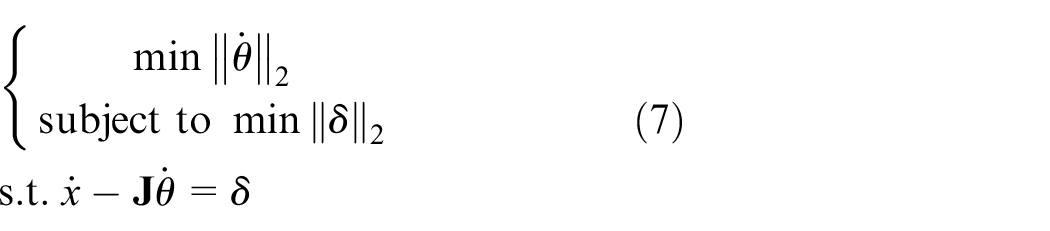
The least solution norm and the least terminal error norm, corresponding to equation (7), can be expressed as

$$\begin{array}{c}\multicolumn{1}{c}{\Vert \stackrel{·}{\theta }{\Vert }_2=\Vert {\mathbf{J}}^{+}\stackrel{·}{x}{\Vert }_2=\Vert \mathbf{V}{\mathbf{\Sigma }}_m^{\mathbf{+}}{\mathbf{U}}^T\stackrel{·}{x}{\Vert }_2}\\ \multicolumn{1}{c}{=\sqrt{{\stackrel{·}{x}}^T\mathbf{U}{\left({\mathbf{\Sigma }}_m^{+}\right)}^2{\mathbf{U}}^T\stackrel{·}{x}}=\sqrt{\sum _{i=1}^m\frac{{\chi }_i^2}{{\sigma }_i^2}}}\end{array}$$

(8)

$$\Vert \delta {\Vert }_2=\Vert \stackrel{·}{x}-\mathbf{J}\stackrel{·}{\theta }{\Vert }_2=\Vert \stackrel{·}{x}-\mathbf{J}{\mathbf{J}}^{+}\stackrel{·}{x}{\Vert }_2=0$$

(9)

where $[{\chi }_1,\dots ,{\chi }_m{]}^T={\mathbf{U}}^T\stackrel{·}{x}$ and other parameters are defined as above.

SRIM

The classical SRIM, also known as the damped least squares method, ¹² has improved the membership of the minimum norm and least squares in the optimization target in equation (7) to be a parallel relationship. Both can be balanced by employed damping factor λ. Therefore, a new optimization target function is constructed as follows

$$\mathrm{G}{\left(\stackrel{·}{\theta }\right)}_{\lambda }=\Vert \stackrel{·}{x}-\mathbf{J}\stackrel{·}{\theta }{\Vert }_2^2+\lambda \Vert \stackrel{·}{\theta }{\Vert }_2^2$$

(10)

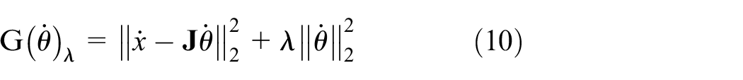
Then, the optimization of the solution of equation (1) can be expressed as

$$\begin{array}{c}\underset{\stackrel{·}{\theta }}{min}\Vert \stackrel{·}{x}-\mathbf{J}\stackrel{·}{\theta }{\Vert }_2^2+\lambda \Vert \stackrel{·}{\theta }{\Vert }_2^2\hfill \\ \mathrm{s}.\mathrm{t}.\stackrel{·}{x}-\mathbf{J}\stackrel{·}{\theta }=\delta \hfill \end{array}$$

(11)

The solution norm $||{\stackrel{·}{\theta }}_{\lambda }|{|}_2$ and the terminal error norm $||{\delta }_{\lambda }|{|}_2$ with damping factor λ are expressed respectively as

$$\begin{array}{c}\multicolumn{1}{c}{\Vert {\stackrel{·}{\theta }}_{\lambda }{\Vert }_2=\Vert {\mathbf{J}}_{\lambda }^{*}\stackrel{·}{x}{\Vert }_2=\Vert {\mathbf{J}}^T{(\mathbf{J}{\mathbf{J}}^T+\lambda \mathbf{E})}^{-1}\stackrel{·}{x}{\Vert }_2}\\ \multicolumn{1}{c}{=\sqrt{\sum _{i=1}^m\frac{{\sigma }_i^2{\chi }_i^2}{{({\sigma }_i^2+\lambda )}^2}}}\end{array}$$

(12)

$$\begin{array}{c}\multicolumn{1}{c}{\Vert {\delta }_{\lambda }{\Vert }_2=\Vert \stackrel{·}{x}-{\mathbf{JJ}}_{\lambda }^{*}\stackrel{·}{x}{\Vert }_2=\Vert \stackrel{·}{x}-\mathbf{J}{\mathbf{J}}^T{(\mathbf{J}{\mathbf{J}}^T+\lambda \mathbf{E})}^{-1}\stackrel{·}{x}{\Vert }_2}\\ \multicolumn{1}{c}{=\sqrt{{\sum _{i=1}^m\left(\frac{\lambda }{{\sigma }_i^2+\lambda }\right)}^2{\chi }_i^2}}\end{array}$$

(13)

with the parameters defined as above. From the formula (12), it can be seen that the introduction of the damping factor λ can keep the norm $||{\stackrel{·}{\theta }}_{\lambda }|{|}_2$ within a reasonable range when the least singular value σ_m tends to 0. For a full-row rank matrix, the terminal error norm of the M-P inverse solution $||\delta |{|}_2=0$ , while $||{\delta }_{\lambda }|{|}_2$ is no longer 0 in formula (13). Therefore, the introduction of damping factor λ eliminates the singularity of the manipulator but increases the terminal error.

Iterative solving process

The inverse motion solutions based on the Jacobian matrix essentially constitute an iterative process, in which the angular variation can only be solved in a stepwise fashion. ²⁷ The main procedural steps are as follows

1. The pose difference value (Δx) is calculated based on the initial pose (x_t) of the current moment and the desired pose (x_t+1) of the next moment; Δx = x_t+1 – x_t.

2. According to the inverse solution formula (5), the corresponding joint angle change $\mathrm{\Delta }\theta$ . is calculated: Δθ = J^*Δx.

3. The joint angle ${\theta }_{t+1}^{*}$ is calculated at the next moment: ${\theta }_{t+1}^{*}={\theta }_t+\mathrm{\Delta }\theta$ .

4. The actual position $(x_{t+1}^{*})$ of the end at the next moment is calculated by the positive kinematics formula: $x_{t+1}^{*}=f({\theta }_{t+1}^{*})$ .

5. The end error $||\delta |{|}_2$ is calculated by $||\delta |{|}_2=||x_{t+1}-x_{t+1}^{*}|{|}_2$ , and is used to determine whether the accuracy requirement is met. If it is, the calculated value is used as the initial value to solve the next point; if not, the parameters are adjusted to calculate a new Jacobian matrix.

Thus, in Step (2), the following approximation formulas should be used

$$\mathrm{\Delta }\theta {|}_{t_k}^{t_{k+1}}=\underset{t_k}{\overset{t_{k+1}}{\int }}{\mathbf{J}}^{*}\stackrel{·}{x}\approx {\mathbf{J}}_{t_k}^{*}\underset{t_k}{\overset{t_{k+1}}{\int }}\stackrel{·}{x}={\mathbf{J}}_{t_k}^{*}\mathrm{\Delta }x$$

(14)

New singularity-avoidance scheme

In this work, the inverse solution of equation (1) is obtained with an improved numerical method based on SRIM, named ESRIM. The optimization model in ESRIM can be expressed as follows

$$\begin{array}{c}\underset{\stackrel{·}{\theta }}{min}\Vert \stackrel{·}{x}-\mathbf{\alpha }\mathbf{J}\stackrel{·}{\theta }{\Vert }_2^2+\Vert \mathbf{\beta }\stackrel{·}{\theta }{\Vert }_2^2\hfill \\ \mathrm{s}.\mathrm{t}.\stackrel{·}{x}-\mathbf{J}\stackrel{·}{\theta }=\delta \hfill \end{array}$$

(15)

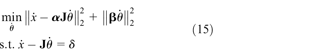
In equation (15), two modified coefficient matrices α and β are introduced, both of which are diagonal matrices

$$\{\begin{array}{c}\mathbf{\alpha }=\mathrm{diag}({\alpha }_1,{\alpha }_2,...,{\alpha }_m)\hfill \\ \multicolumn{1}{c}{\mathbf{\beta }=[\mathrm{diag}({\beta }_1,{\beta }_2,...,{\beta }_m)|0_{m\times (n-m)}]}\end{array}$$

(16)

The damping matrix β replaces the unified damping factor λ of SRIM. A pre-factor matrix α is also added into the target function, in order to eliminate the error caused by the change of singular values when the manipulator passes singular points. The optimization target function is constructed as

$$\begin{array}{c}\multicolumn{1}{c}{G{\left(\stackrel{·}{\theta }\right)}_{\alpha \beta }=\Vert \stackrel{·}{x}-\mathbf{\alpha }\mathbf{J}\stackrel{·}{\theta }{\Vert }_2^2+\Vert \mathbf{\beta }\stackrel{·}{\theta }{\Vert }_2^2}\\ \multicolumn{1}{c}{=\left[\begin{array}{cc}{(\stackrel{·}{x}-\mathbf{\alpha }\mathbf{J}\stackrel{·}{\theta })}^T\hfill & {\stackrel{·}{\theta }}^T\hfill \end{array}\right]\left[\begin{array}{cc}{\mathbf{E}}_{m\times m}\hfill & 0\hfill \\ \multicolumn{1}{c}{0}& {\left({\mathbf{\beta }}^T\mathbf{\beta }\right)}_{n\times n}\hfill \end{array}\right]}\\ \multicolumn{1}{c}{\left[\begin{array}{c}\stackrel{·}{x}-\mathbf{\alpha }\mathbf{J}\stackrel{·}{\theta }\hfill \\ \multicolumn{1}{c}{\stackrel{·}{\theta }}\end{array}\right]}\\ \multicolumn{1}{c}{={(\stackrel{·}{\theta }-{\stackrel{·}{\theta }}_{\alpha \beta })}^T({\mathbf{J}}^T{\mathbf{\alpha }}^T\mathbf{\alpha }\mathbf{J}+{\mathbf{\beta }}^T\mathbf{\beta })(\stackrel{·}{\theta }-{\stackrel{·}{\theta }}_{\alpha \beta })+{\stackrel{·}{x}}^T{\mathbf{W}}_{\alpha \beta }\stackrel{·}{x}}\end{array}$$

(17)

In equation (17)

$${\mathbf{W}}_{\alpha \beta }={\mathbf{E}}_m-\mathbf{\alpha }\mathbf{J}{({\mathbf{J}}^T{\mathbf{\alpha }}^T\mathbf{\alpha }\mathbf{J}+{\mathbf{\beta }}^T\mathbf{\beta })}^{-1}{\mathbf{J}}^T{\mathbf{\alpha }}^T$$

(18)

Since J ^T α ^T αJ + β ^T β is positive definite in the formula (17), $G(\stackrel{·}{\theta }{)}_{\alpha \beta }$ is a positive-definite quadratic form of $\stackrel{·}{\theta }$ and has a minimum value only if $\stackrel{·}{\theta }={\stackrel{·}{\theta }}_{\alpha \beta }$ . Then the solution of formula (1) for optimum configuration (15) is as follows

$${\stackrel{·}{\theta }}_{\alpha \beta }={({\mathbf{J}}^T{\mathbf{\alpha }}^T\mathbf{\alpha }\mathbf{J}+{\mathbf{\beta }}^T\mathbf{\beta })}^{-1}{\mathbf{J}}^T{\mathbf{\alpha }}^T\stackrel{·}{x}$$

(19)

The extended singular robust inverse of the Jacobian matrix corresponding to equation (19) is

$${\mathbf{J}}_{\alpha \beta }^{*}={({\mathbf{J}}^T{\mathbf{\alpha }}^T\mathbf{\alpha }\mathbf{J}+{\mathbf{\beta }}^T\mathbf{\beta })}^{-1}{\mathbf{J}}^T{\mathbf{\alpha }}^T$$

(20)

Furthermore, J*_αβ can be expressed as a simple calculation, ¹⁶ as follows

$${\mathbf{J}}_{\alpha \beta }^{*}={\mathbf{J}}^T{\mathbf{\alpha }}^T{(\mathbf{\alpha }\mathbf{J}{\mathbf{J}}^T{\mathbf{\alpha }}^T+\mathbf{\beta }{\mathbf{\beta }}^T)}^{-1}$$

(21)

Then, for any Jacobian matrix J, the minimum norm $||{\stackrel{·}{\theta }}_{\alpha \beta }|{|}_2$ and the end error $||{\stackrel{·}{\delta }}_{\alpha \beta }|{|}_2$ of the extended singularly robust inverse solution are

$$\begin{array}{c}\multicolumn{1}{c}{\Vert {\stackrel{·}{\theta }}_{\alpha \beta }{\Vert }_2=\Vert {\mathbf{J}}_{\alpha \beta }^{*}\stackrel{·}{x}{\Vert }_2}\\ \multicolumn{1}{c}{=\Vert {\mathbf{J}}^T{\mathbf{\alpha }}^T{(\mathbf{\alpha }\mathbf{J}{\mathbf{J}}^T{\mathbf{\alpha }}^T+\mathbf{\beta }{\mathbf{\beta }}^T)}^{-1}\stackrel{·}{x}{\Vert }_2}\end{array}$$

(22)

$$\begin{array}{c}\multicolumn{1}{c}{\Vert {\delta }_{\alpha \beta }{\Vert }_2=\Vert \stackrel{·}{x}-{\mathbf{JJ}}_{\alpha \beta }^{*}\stackrel{·}{x}{\Vert }_2}\\ \multicolumn{1}{c}{=\Vert \stackrel{·}{x}-\mathbf{J}{\mathbf{J}}^T{\alpha }^T{(\alpha \mathbf{J}{\mathbf{J}}^T{\alpha }^T+\beta {\beta }^T)}^{-1}\stackrel{·}{x}{\Vert }_2}\end{array}$$

(23)

The approximate modified Jacobian matrix J _α  = αJ(θ) is called the truth Jacobian matrix. Equation (4) can be expressed as

$$\mathrm{\Delta }x={\mathbf{J}}_{\alpha }\left(\theta \right)\mathrm{\Delta }\theta$$

(24)

The pre-factor matrix α is introduced to correct the approximation of the Jacobian matrix at t_k+1. For the ith axis, it is reasonable to approximate the correction coefficient α_i from the change of σ_i during the time interval, which is the ith singular value of the Jacobian matrix. In this work, the pre-factors are calculated as follows

$${\alpha }_i=\frac{{\alpha }_0}{2}*\left(\frac{{\sigma }_i^{t_{k-1}}+{\sigma }_i^{t_k}}{{\sigma }_i^{t_k}}\right),i=1,2,\dots ,m$$

(25)

where α₀ is an adjustable critical pre-factor. In order to prevent the singularity caused by the small singular values of the matrix, the truth Jacobian matrix J _α is improved by adding the damping matrix β, and the modified Jacobian matrix is denoted as J _αβ . Introducing β gives rise to an inevitable computational error δ(J _α ), which is expressed as

$$\delta \left({\mathbf{J}}_{\alpha }\right)={\mathbf{J}}_{\alpha \beta }-{\mathbf{J}}_{\alpha }$$

(26)

The relative error $\delta \left(\mathrm{\Delta }\theta \right)/\mathrm{\Delta }\theta$ of the solution of equation (15) satisfies the following formula

$$\frac{\delta \left(\mathrm{\Delta }\theta \right)}{\mathrm{\Delta }\theta }\le \frac{\Vert {\mathbf{J}}_{\alpha }^{*}\Vert \Vert {\mathbf{J}}_{\alpha }\Vert \frac{\Vert \delta \left({\mathbf{J}}_{\alpha }\right)\Vert }{\Vert {\mathbf{J}}_{\alpha }\Vert }}{1-\Vert {\mathbf{J}}_{\alpha }^{*}\Vert \Vert {\mathbf{J}}_{\alpha }\Vert \frac{\Vert \delta \left({\mathbf{J}}_{\alpha }\right)\Vert }{\Vert {\mathbf{J}}_{\alpha }\Vert }}$$

(27)

When the value $||{\mathit{J}}_{\alpha }^{*}||||\delta ({\mathit{J}}_{\alpha })||<1$ , the selection of β should minimize $\underset{\beta }{min}||{\mathit{J}}_{\alpha }^{*}||||{\mathit{J}}_{\alpha \beta }-{\mathit{J}}_{\alpha }||$ , and this goal formula can be transformed as

$$\begin{array}{c}\multicolumn{1}{c}{\Vert J_{\alpha }^{*}\Vert \Vert J_{\alpha \beta }-J_{\alpha }\Vert =\Vert J_{\alpha }^{*}\Vert \Vert {\left(J_{\alpha }^T\right)}^{*}({J_{\alpha }}^T{J}_{\alpha }+{\beta }^T\beta )-J_{\alpha }\Vert }\\ \multicolumn{1}{c}{=\Vert J_{\alpha }^{*}\Vert \Vert {\left(J_{\alpha }^T\right)}^{*}{\beta }^T\beta \Vert }\end{array}$$

(28)

Obviously, when β_i = 0 (i = 1, 2,…, r), formula (28) reaches its minimum value of 0. A non-zero value of β_i helps avoid the singularity caused by small singular values, but it also leads to a larger terminal error. In this work, β_i is defined as a piecewise function of σ_i as follows

$${\beta }_i=\{\begin{array}{c}\sqrt{{\sigma }_0^2-{{\sigma }_i}^2}\mathrm{for}{\sigma }_i\le {\sigma }_0\hfill \\ \multicolumn{1}{c}{0\mathrm{for}{\sigma }_i>{\sigma }_0}\end{array}$$

(29)

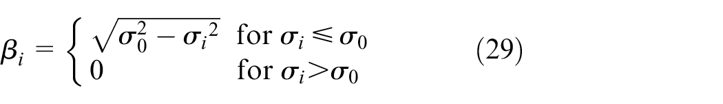
where i = 1, 2,…, m, and σ₀ is the smallest singular value allowed. Equation (29) avoids the terminal error caused by over-optimization when singular values are large enough.

For the full-row rank Jacobian matrix J, the least norm $||{\theta }_{\alpha \beta }|{|}_2$ and the terminal error norm $||{\delta }_{\alpha \beta }|{|}_2$ of the extended singular robust inverse solution can be reduced to

$$\begin{array}{c}\multicolumn{1}{c}{\Vert {\stackrel{·}{\theta }}_{\alpha \beta }{\Vert }_2=\sqrt{\sum _{i=1}^m{\left(\frac{{\sigma }_i}{{\sigma }_i^2+{{\beta }_i}^2}\right)}^2{\chi }_{\alpha i}^2}}\\ \multicolumn{1}{c}{=\sqrt{\sum _{i=1}^j{\left(\frac{{\sigma }_i}{{\sigma }_0^2}\right)}^2{\chi }_{\alpha i}^2+\sum _{i=j+1}^m{\left(\frac{1}{{\sigma }_i}\right)}^2{\chi }_{\alpha i}^2}}\end{array}$$

(30)

$$\begin{array}{c}\multicolumn{1}{c}{\Vert {\delta }_{\alpha \beta }{\Vert }_2=\sqrt{{\sum _{\mathrm{i}}^m\left(\frac{{{\beta }_i}^2}{{\sigma }_i^2+{{\beta }_i}^2}\right)}^2{\chi }_{\alpha i}^2}}\\ \multicolumn{1}{c}{=\sqrt{{\sum _{\mathrm{i}=1}^j\left(\frac{{\sigma }_0^2-{\sigma }_i^2}{{\sigma }_0^2}\right)}^2{\chi }_{\alpha i}^2}}\end{array}$$

(31)

where $[{\chi }_{\alpha 1},\dots ,{\chi }_{\alpha m}{]}^T={\mathbf{U}}^T{\mathbf{\alpha }}^{-1}\stackrel{·}{x}$ , σ_j satisfies σ_j ≤ σ₀ and σ_j+1 > σ₀. The inverse solution obtained by ESRIM takes the current singular value of the Jacobian matrix into account, and the overlarge value of $||{\theta }_{\alpha \beta }|{|}_2$ near the singular point is numerically avoided. In addition, the solution dose not exhibit over-optimization error.

In the process of trajectory tracking, with the solution error, $\stackrel{·}{\theta }$ can finally be expressed as

$$\stackrel{·}{\theta }={\stackrel{·}{\theta }}_{\alpha \beta }+{\stackrel{·}{\theta }}_{\delta }={\mathbf{J}}_{\alpha \beta }^{*}{\stackrel{·}{x}}_d+{\mathbf{J}}_{\alpha \beta }^{*}{\delta }_{\alpha \beta }$$

(32)

The stability of the proposed method is also analyzed. According to the stability criterion,^28–30 the Lyapunov function ²⁹ is defined as

$$V=\frac{1}{2}{\delta }_{\alpha \beta }^T{K}_i{\delta }_{\alpha \beta }+\frac{1}{2}{\stackrel{·}{\theta }}_{\alpha \beta }^T{K}_p{\stackrel{·}{\theta }}_{\alpha \beta }$$

(33)

Then, there are

$$\begin{array}{c}\multicolumn{1}{c}{\stackrel{·}{V}={\delta }_{\alpha \beta }^T{K}_i{\stackrel{·}{\delta }}_{\alpha \beta }+{\stackrel{·}{\theta }}_{\alpha \beta }^T{K}_p{\stackrel{··}{\theta }}_{\alpha \beta }}\\ \multicolumn{1}{c}{={\delta }_{\alpha \beta }^T{K}_i({\stackrel{·}{\mathit{x}}}_d-\stackrel{·}{\mathit{x}})+{\stackrel{·}{\theta }}_{\alpha \beta }^T{K}_p{\stackrel{··}{\theta }}_{\alpha \beta }}\\ \multicolumn{1}{c}{={\delta }_{\alpha \beta }^T{K}_i{\stackrel{·}{\mathit{x}}}_d-{\delta }_{\alpha \beta }^T{K}_i{\mathbf{J}}_{\alpha \beta }{\stackrel{·}{\theta }}_{*}+{\stackrel{·}{\theta }}_{\alpha \beta }^T{K}_p{\stackrel{··}{\theta }}_{\alpha \beta }}\\ \multicolumn{1}{c}{=-{\delta }_{\alpha \beta }^T{K}_i{\delta }_{\alpha \beta }+{\stackrel{·}{\theta }}_{\alpha \beta }^T{K}_p{\stackrel{··}{\theta }}_{\alpha \beta }}\end{array}$$

(34)

where K_i and K_p are both positive constant coefficients and are determined by the actual speed. V is always positive definite. Whether positive or not, $\stackrel{·}{V}$ determines the stability of the proposed method. Obviously, we can choose the appropriate values of α₀ and σ₀, which make up of α and β, to satisfy the stability requirement of $\stackrel{·}{V}$ as negative definite.

Simulation analysis verification

Taking the 7-axis manipulator “YL101” (designed in our laboratory) as the object, the effects of ESRIM are studied and compared with those of SGIM and SRIM; the latter are well known as traditional methods providing good inverse solutions of trajectory tracking.

“DH” method was first proposed by Denavit and Hartenberg. ³¹ It is the most common and mature method to describe the structure of chain manipulator. ³² The structure of the 7-axis manipulator “YL101” is shown in Figure 1 and the DH structural parameters are listed in Table 1.

Figure 1.

Structural diagram of “YL101” 7-axis manipulator.

Table 1.

DH structural parameters of “YL101” manipulator.

θ	d (mm)	a (mm)	α (°)
θ 1	105	0	90°
θ 2	0	500	0
θ 3	0	274	−90
θ 4	0	198.5	90°
θ 5	0	198.5	−90°
θ 6	0	195	90°
θ 7	236	0	0°

Example 1: linear trajectory

In the first simulation example, the tracking trajectory of the manipulator is a spatial straight line L_S, ranging from the initial point S_p (982.9, −399.6, and −324.3 mm) to the end point E_p (394.5, −399.9, and −441.4 mm), and with the corresponding RPY ³³ attitude angle ranging from S_a (–45.0°, 37.6°, and 49.3°) to E_a (–42.4°, 148.8°, and −163.8°). The established end precision requires that the position be controlled to within 0.5 mm. K_i and K_p are 1.0 and 0.125, respectively.

As a result of the accuracy requirement, the step size is set as 0.05 mm. The SGIM has no specific parameter settings. In SRIM, the damping coefficient is set as $\lambda ={\lambda }_0||\delta |{|}^2$ according to the recommendation of Chan and Lawrence, ¹⁹ and ${\lambda }_0=2.22$ to achieve the best results. In the proposed ESRIM calculation, the critical pre-factor and singular value are α₀ = 2.30 and σ₀ = 2.75, respectively. The simulation results are shown in Figures 2–7.

Figure 2.

Terminal errors of different optimizing methods in spatial linear trajectory (a of the first singular point, b of the second singular point).

Figure 3.

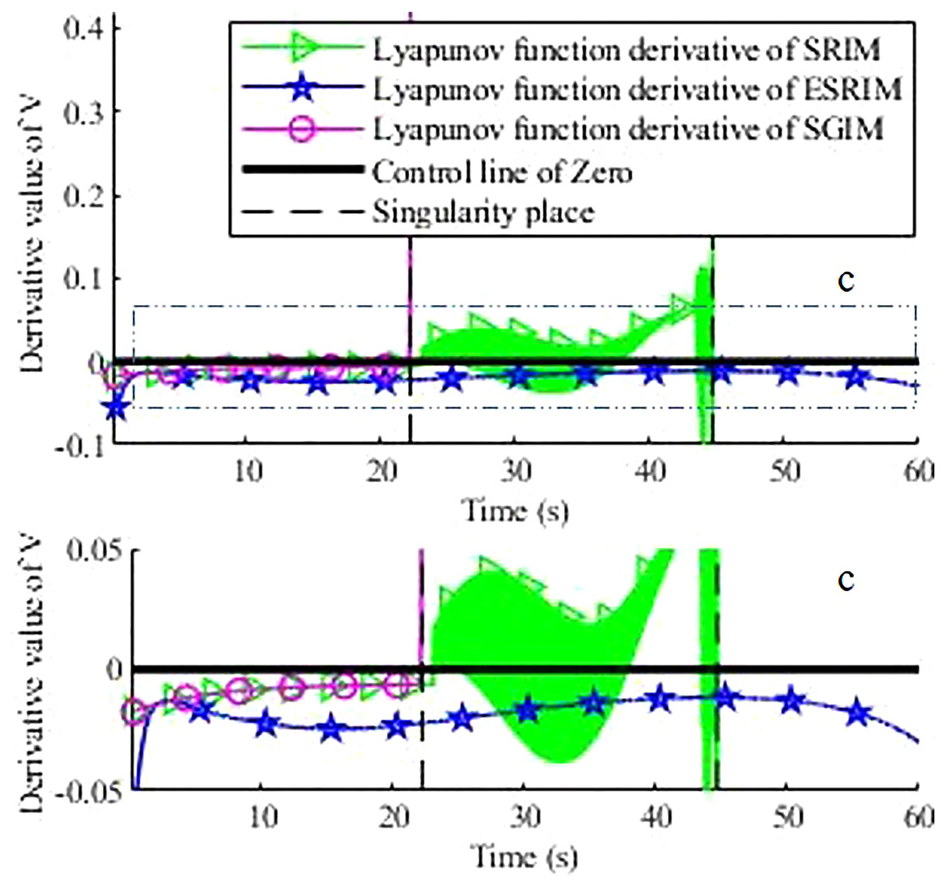
Lyapunov objective function derivative values with different optimizing methods in spatial linear trajectory (c of V derivative values in enlarged area).

Figure 4.

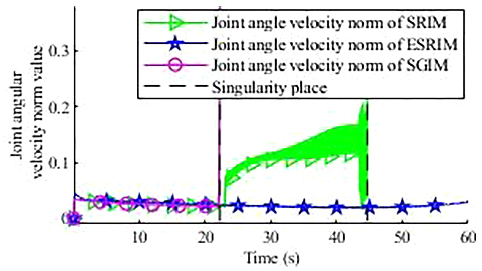
Joint angular velocity norm of different optimizing methods in spatial linear trajectory.

Figure 5.

Least singular value of different optimizing methods in spatial linear trajectory.

Figure 6.

Position and posture changes of different optimizing methods in spatial linear trajectory (a) SGIM, (b) SRIM, and (c) ESRIM.

Figure 7.

Joint angles value of ESRIM methods in spatial linear trajectory.

The terminal errors resulting from the three different methods are compared in Figure 2. Before the manipulator moves close to the first singular point, all three methods obtain good trajectories with acceptable small terminal errors. However, only ESRIM smoothly finds the solution over the entire process. Figure 2(a) shows the vicinity of the first singular point S_P1. When the manipulator approaches S_P1, the terminal error of the SGIM solution oscillates rapidly and then diverges until it exceeds the allowable error value; this leads to the failure of the whole optimization process. Adding the damping factor λ allows SRIM to find the solution around S_P1. However, large oscillation occurs in the subsequent SRIM solution, and this violates the accuracy requirement around point S_P2 (Point b in Figure 2). Compared with the former two methods, ESRIM obtains the solutions of S_P1 and S_P2 simultaneously. The terminal error does not exhibit oscillation with long duration or large amplitude and shows better optimization performance as the optimization process continues.

Figure 3 shows the Lyapunov objective function derivative values $\stackrel{·}{V}$ for the different optimizing methods. $\stackrel{·}{V}$ should be negative, which is necessary for the stability of the optimization process. Before the first singular point, the $\stackrel{·}{V}$ values of the three methods are all negative definite. However, the values of SGIM and SRIM oscillate and turn positive and eventually lead to the failure of the subsequent iteration process. Only the proposed ESRIM maintains the negative $\stackrel{·}{V}$ and satisfies the stability requirement.

In addition to the optimization of terminal error, the norm of joint angular velocity should be small enough to be practical. As shown in Figure 4, the joint angular velocity for SGIM increases rapidly at the singular point S_P1, and this is consistent with the variation in its error. The same relationship can be observed for joint angular velocity and terminal error with SRIM. Compared with SGIM and SRIM, the joint angular velocity of the proposed ESRIM is much more stable and remains a low level even at both of the singular points.

Equation (8) indicates that smaller singular values will lead to larger joint angular velocity and reduced flexibility of the manipulator. Therefore, for a certain terminal position, the least singular value σ_m of the Jacobian matrix should be as large as possible. Figure 5 shows the variation of the least singular values with the three optimization methods, and ESRIM produces the largest σ_m during the entire iteration process. These results show that ESRIM improves the flexibility of the manipulator.

Figure 6 shows the track of the manipulator when different optimization methods are used to produce a spatial linear trajectory. The three tracks are generally consistent, but only the ESRIM successfully passes both singular points and completes the whole trajectory.

In addition, Figure 7 shows the trends in the angles of each joint during the optimization with ESRIM. All the joint angles change smoothly without sharp variations, and they remain within the range limits.

Example 2: curve trajectory

In the second example, the tracking trajectory is set as a spatial arc L_C1, ranging from the initial point S_p (1080.6, 89.7, and 752.7 mm) to the end point E_p (632.1, 89.7, and 970.9 mm) with the corresponding RPY attitude angle ranging from S_a (−46.7°, 123.7°, and −147.9°) to E_a (−123.0°, 106.7°, and −93.0°). The end precision is limited to 0.5 mm of the target position, with circle center of O_C (830.3, 457.1, and 1065.2) and normal vector of n_c (0, –1, 0).

Because of the accuracy requirements, the arc-length step size is set as 0.05 mm. SGIM has no specific parameter settings. In SRIM, the parameters are set as $\lambda ={\lambda }_0||\delta |{|}^2$ , where λ₀ = 1.8 can achieve the best results. The parameters of ESRIM are set as α₀ = 2.1 and σ₀ = 0.5. The simulation results are shown in Figures 8 and 9.

Figure 8.

Simulation results of 7-axis manipulator with different optimizing methods in spatial arc trajectory: (a) terminal error value of different optimizing methods, (b) joint angular velocity norm value of different optimizing methods, (c) least singular value of different optimizing methods, and (d) position and posture changes of ESRIM.

Figure 9.

Lyapunov objective function derivative values with different optimizing methods in spatial arc trajectory (d of V derivative values in enlarged area).

As with straight lines, tracking trajectories of spatial curves are also among the most common basic tasks. Taking arc trajectory L_C1 as an example, the optimization results with SGIM, SRIM, and ESRIM are studied. As compared with straight lines, tracking spatial curves are more difficult. From Figure 8, it can be seen that the singularity of SGIM occurs shortly after the simulation begins. At the singular point, the terminal error breaks through the allowed limit and the tracking fails. SRIM with a damping factor passes through the initial singularity, but the terminal error oscillates severely during the iteration process. When approaching the next singularity point, the terminal error experiences a sharp divergent oscillation and this leads to tracking failure. However, ESRIM optimization exhibits the best result. Generally, ESRIM obtains lower joint angular velocities and larger singular values, corresponding to better practicability and flexibility. As with the results in Example 1, the terminal error of ESRIM is sometimes higher than SGIM and SRIM, but the error still meets the accuracy requirement. Moreover, only ESRIM passes through both two singular points successfully and obtains joint angle solutions during the whole curve-tracking process. As shown in Figure 9, only the Lyapunov derivative value of ESRIM is negative and satisfies the stability requirement. It can be seen that ESRIM again exhibits better optimization performance in this curve trajectory tracking for the 7-axis manipulator.

Example 3: 10-axis manipulator

In this example, the 7-axis is replaced with a multi-axis redundant manipulator to validate the performances of the different methods. The DH structure parameters of the 10-axis manipulator are listed in Table 2.

Table 2.

DH structural parameters of 10-axis manipulator.

θ	d (mm)	a (mm)	α (°)
θ 1	105	0	90°
θ 2	0	500	0
θ 3	0	274	−90°
θ 4	0	198.5	90°
θ 5	0	198.5	−90°
θ 6	0	198.5	90°
θ 7	0	198.5	−90°
θ 8	0	198.5	90°
θ 9	0	195	−90°
θ 10	236	0	0°

The optimization is applied to spatial arc curve L_C2, the RPY attitude angle extends from S_a (84.5°, 84.0°, and 90.4°) to E_a (120.6°, 40.9°, and 140.8°), and other parameters are the same as those described in Example 2. The arc-length step size is also set to 0.05 mm. The parameters of SRIM are set as λ₀ = 0.01 and the parameters of ESRIM are α₀ = 1.7 and σ₀ = 1.3. The simulation results are shown in Figures 10 and 11.

Figure 10.

Lyapunov objective function derivative values of 10-axis manipulator with different optimizing methods in spatial linear trajectory (e of V derivative values in enlarged area).

Figure 11.

Simulation results for 10-axis manipulator with different optimizing methods in a spatial arc trajectory: (a) terminal error value of different optimizing methods, (b) joint angular velocity norm value of different optimizing methods, (c) least singular value of different optimizing methods, and (d) position and posture changes of ESRIM.

As with the 7-axis manipulator, the SGIM solution for the 10-axis manipulator also becomes singular near the beginning of the simulation. SRIM fails to perform better than does SGIM in the tracking process for trajectory L_C2, while the proposed ESRIM performs well. In the limited range, the terminal error is smooth and continuous, and no overall oscillation occurs. The least singular value at the same position is the largest while the joint angular velocity is the smallest. Therefore, the ESRIM shows better optimization performance for the multi-axis redundant manipulator. In addition, the Lyapunov derivative value of ESRIM is negative, which is as expected.

Conclusion

The conclusions of this study are as follows:

1. To address the problem that the manipulator’s singularity of different joints cannot be adjusted separately by the classical SRIM, a scheme in which the damping factor matrix β replaces the unified damping coefficient λ is proposed. To address the Jacobian matrix approximation error, which usually exists in the iterative control optimization process, the correction coefficient matrix α is employed and the ESRIM is formed.

2. Large values of manipulator terminal error and joint angular velocity, caused by the singularities in three optimization methods are analyzed, and the semi-empirical selection principle of β and α is given. Furthermore, the stability of the proposed method is investigated with reference to the Lyapunov stability criteria.

3. Three simulation methods are compared in the tracking of spatial straight lines and curved trajectories. The simulation results show that the ESRIM exhibits better optimization performance and stability as the process continues. In the prescribed range, the terminal error does not show oscillation with longer duration or large amplitude. Meanwhile, under the same conditions, the least singular value of ESRIM is the largest and the joint angular velocity is the smallest, which is as expected.

4. The different optimized methods have also been applied with a 10-axis manipulator, and positive results are obtained with ESRIM; this indicates that the extended robust inverse method for multi-axis redundant manipulators has broad applicability and can avoid singularity. However, it should be noted that all three methods based on singular value decomposition of the Jacobian matrix require long calculation times, which is deserved to research and this should be investigated and improved in future work.