
Abstract
In this article, the space-time conservation element and solution element scheme is extended to simulate the unsteady compressible two-phase flow in pipes. The model is non-conservative and the governing equations consist of three equations, namely, two mass conservation equations for each phase and one mixture-momentum equation. In the third equation, the non-conservative source term appears, which describes the sum of gravitational and frictional forces. The presence of source term and two mass conservation equations in considered model offers difficulties in developing the accurate and robust numerical techniques. The suggested space-time conservation element and solution element numerical scheme resolves the volume-contact discontinuities efficiently. Furthermore, the modified central upwind scheme is also extended to solve the same two-phase flow model. The number of test problems is considered, and the results obtained by space-time conservation element and solution element scheme are compared with the solutions of modified central upwind scheme. The numerical results show better performance of the space-time conservation element and solution element method as compare to the modified central upwind scheme.
Keywords
Introduction
Two-phase flows are widely observed in natural environment, such as snowy or rainy winds, typhoons, water and air pollution, and volcanic eruptions. They are also extensively encountered in nuclear power plants, combustion engines, bio-medical engineering, food processing industry, and many more.1–3 Because of these wide range applications, many researchers had developed several two-phase models and numerical methods to study the dynamics of such flows. These two-phase flow models inherit several numerical difficulties since each phase is considered separately and the model comprises two sets of conservation of mass, momentum, and energy. For example, the presence of two momentum equations causes difficulties such as loss of hyperbolicity and uncertainties in specifying interfacial interaction terms between the two phases. Here, we are interested in the model that elaborates the compressible two-phase flow in gas and liquid horizontal pipelines. However, above-mentioned difficulties in two-phase flow models are remarkably reduced by formulating the drift-flux model, in which the mixture momentum equation is utilized to describe the motion of whole mixture. This model is a powerful tool for gaining insight into the flow processes where oil and gas are transported simultaneously out of a reservoir. Without modeling of such flows in oil industry, it is very difficult to describe effects that may arise within a well bore over time to weaken or improve production.
In this article, we consider the drift-flux model 4 that consists of two mass conservation equations for each phase and one momentum equation for the mixture. The drift-flux model was initially designed by Zuber and Findlay 5 and has been improved by many researchers.4,6– 9 The considered drift-flux model is derived from the two-fluid model by adding the two momentum equations for each phase. 10 Now, more difficult terms associated with phase interaction are canceled out, and the missing information is obtained using the kinematic constitutive equation, 7 which relates the phase velocities at any point. Still, the source term that is sum of gravitational and frictional forces is presented in the considered model. This model explains the isothermal liquid-gas flow in the long pipeline where the flow behavior is averaged and perpendicular to the pipe axis. Hence, the resulting model is one-dimensional (1D) in the direction of axis.
Due to importance of the drift-flux model, many numerical schemes had been designed and extended to investigate this model in the literature. First of all, Romate 6 has developed an approximate Roe-type Riemann solver for computing the drift-flux model. Afterward, hybrid flux-splitting and relaxation-type numerical schemes are designed to solve the same model in Evje and Fjelde,7,11 respectively. Meanwhile, Fjelde and Karlsen 4 have developed high-resolution hybrid upwind scheme to analyze the considered model. In this scheme, for a smooth region, a simple non-conservative Monotonic Upwind Scheme for Conservation Laws (MUSCL) scheme and, in a region of strong discontinuities, high-resolution conservative scheme are utilized. Next, in Evje and Fjelde, 12 another splitting method, namely, advection upstream splitting method, is extended to analyze the drift-flux model. 7 Furthermore, for solving the same model, semi-implicit relaxation scheme is proposed in Baudin et al. 8 and a numerical scheme weakly implicit mixture flux (WIMF) is extended in Steinar et al. 13 Subsequently, the multi-stage approach (MUSTA) is used to develop the centered numerical scheme for investigating the drift-flux model in Munkejord et al. 9 Recently, Paula and Valdes 14 analyze the drift-flux model in two-phase slug-flow in horizontal and inclined pipelines using experimental non-Newtonian and Newtonian approaches.
In this article, the space-time conservation element and solution element (CE/SE) scheme 15 is extended for simulating the compressible two-phase flow in horizontal oil and gas pipelines. This scheme is entirely different from the schemes which have been applied before to solve the considered model. This method has many distinct features, such as treatment of space and time at the same step, introduction of conservation elements (CEs) and solution elements (SEs), shock capturing approach without utilizing Riemann solvers, and the use of staggered grid. Besides these distinct features, the suggested scheme is distinguished by the simplicity of its conceptual basis-conservation of flux in time and space; for details, see Chang. 15 Various applications of CE/SE scheme in different areas affirm the scheme’s generality, robustness, and effectiveness.15–24 Later on, H Shen and colleagues25,26 designed a new upwind CE/SE scheme which is based on the “a” scheme (the original CE/SE scheme). In this new scheme, the numerical dissipation is added through the upwind procedure. This upwind CE/SE scheme preserves almost all features of the original CE/SE scheme. For extensive detail, the reader is referred to the literature.27–31 The number of test problems is considered to show that the suggested scheme is highly robust, gives better resolutions of the sharp volume-fraction contact discontinuities, and preserves the positivity of flow variables such as fluid densities, volume fractions, and pressure. For checking the accuracy of proposed numerical scheme, we have extended the modified central upwind scheme (CUP) 32 for solving the considered drift-flux model, and the results obtained from CE/SE scheme are compared with those of modified CUP.
The rest of article is organized as follows. In section “Drift-flux model,” the drift-flux model is given and data-dependent terms are described. The CE/SE scheme for drift-flux model is described in section “Construction of CE/SE scheme for 1D drift-flux model.” In section “Numerical test problems,” different interesting test problems are included, to validate and compare the results of suggested numerical schemes. Finally, a conclusion of this article is drawn in section “Conclusion.”
Drift-flux model
In this section, we present the mathematical form and eigen-structure of the drift-flux model. Also, we describe the submodels that are used in this article. We will restrict ourselves to consider liquid-gas isothermal flow in the horizontal pipeline. The fundamental equations for the considered drift-flux model are written as

Here,

Here,

The considered model contains seven unknowns
1. Volume fractions are related by the following relation

2. We use submodel for density of liquid as

and submodel for density of gas as follows
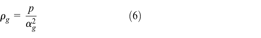
Here,
3. We use the following algebraic form of gas slip relation for computational purposes

Here,
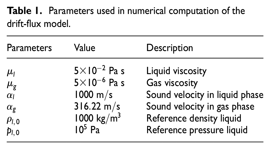
Parameters used in numerical computation of the drift-flux model.
Eigen-structure
The system of equation (1) can be written as

where

with

Note that the passive variable pressure can be obtained from the conservative variables
First, by assuming

The above system is the required expression for finding the Jacobian matrix. Now, by applying the definition of

Using the values of phase densities

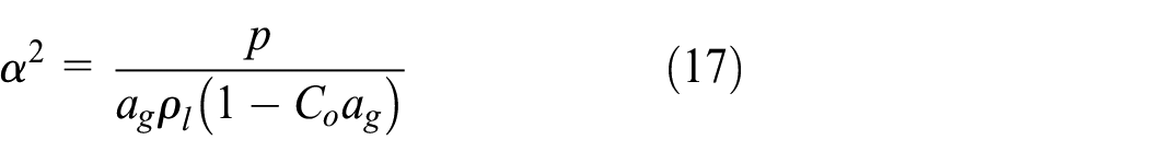
By rearranging equation (12) with respect to pressure

where

Now, from the flux vector in equation (10), we obtain the Jacobian matrix as follows
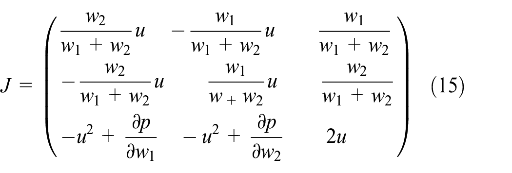
with
Second, we assume that
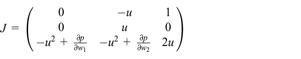
The corresponding eigenvalues are

where
Construction of CE/SE scheme for 1D drift-flux model
The CE/SE numerical has entirely different concept and methodology from the well-established numerical techniques such as the finite difference, finite volume, and finite element methods. In this section, the 1D CE/SE scheme 15 is constructed for 1D drift-flux model (1). For the construction of CE/SE scheme, we rewrite equation (8) in component form as

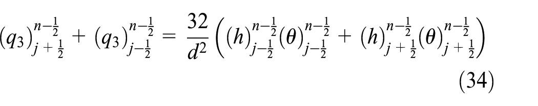
Let

where
We denote the computational domain by

and


Space-time staggered grid near SE (j, n) (a) Space-time staggered grid near SE(j,n), (b) CE_(-)(j,n) and CE_(+)(j,n), and (c) CE(j,n).
Moreover

By employing chain rule, we obtain


where
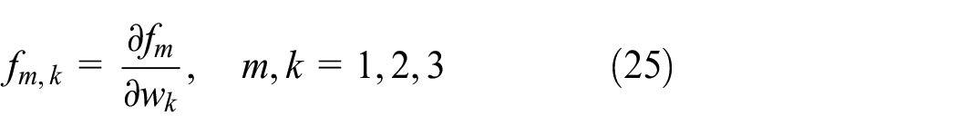
The Jacobian matrix is formed by

Moreover, due to the smoothness assumption of variables for any

Using equations (20) and (21), equation (27) is equivalent to
We notice that
Let
Note that, among the line segments forming the boundary of

According to this equation, the total flux leaving boundary of any BCE is zero. Because the surface integration over any interface separating two neighboring BCEs is evaluated using the information from a single SE, obviously, the local conservation relation (29) leads to a global flux conservation relation, that is, the total flux of
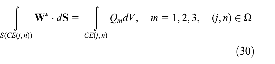
must follow from equation (29).
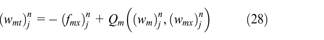
Using equation (29) along with equations (20)–(22) and (26), one obtains

or above equation can be written as
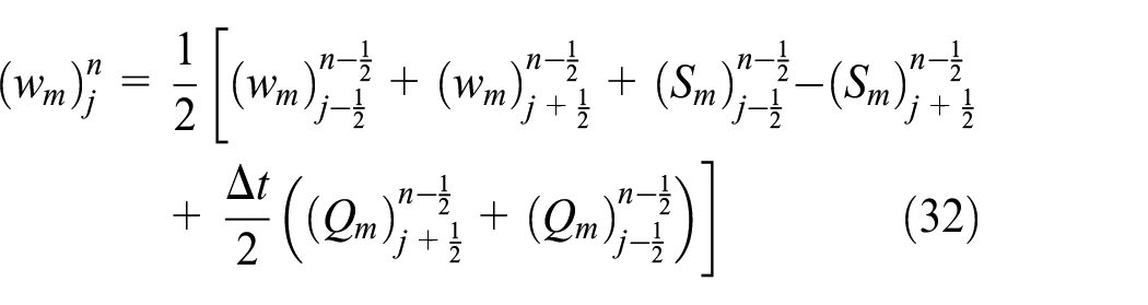
where

Note that
where
The numerical oscillations near a discontinuity can be suppressed using the following limiting formulations for the slopes of conservative variables

Here,

Moreover

and

Equations (32) and (35)–(38) constitute the CE/SE solver for 1D drift-flux model. This completes the construction of proposed solver.
Numerical test problems
In this section, several test problems are presented for the drift-flux flow model. The obtained results of CE/SE scheme are also compared with the results of modified CUP.
32
Furthermore, the reference solutions are obtained using the CE/SE numerical scheme on uniform
The first two test problems are taken from Kuila et al.
34
for checking the accuracy of proposed numerical schemes. Our proposed numerical schemes show better performance in resolving strong discontinuities as compared to the designed numerical schemes in Kuila et al.
34
The pressure
Test problem 1
The left and right states of the Riemann problem are
Here, the subscripts

The solution of Riemann problem at
Test problem 2
The left and right states of the Riemann problem are

The solution profiles of test problem are given in Figure 3 at time

Numerical results of Riemann problem at
The next two test problems are taken from Fjelde and Karlsen.
4
In these problems, we consider the liquid density
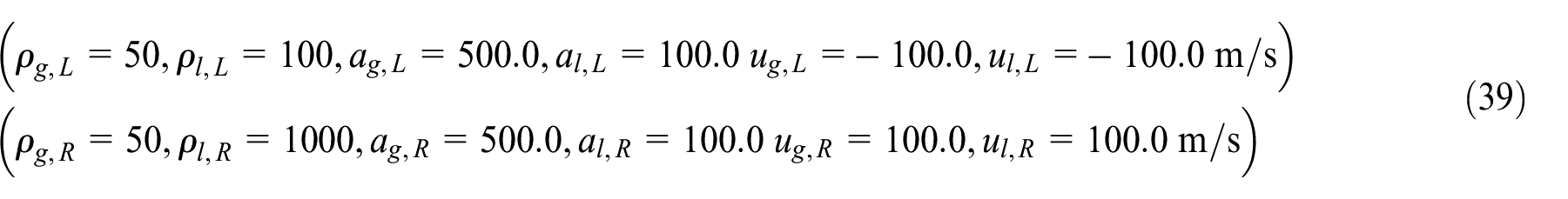
Test problem 3
The left and right states of this Riemann problem are
The solution consists of a left going shock wave, a contact wave, and a right going shock wave, as shown in Figure 4. The results obtained by different schemes at time
Numerical results of Riemann problem by CE/SE and CUP schemes at t = 1.0 s.
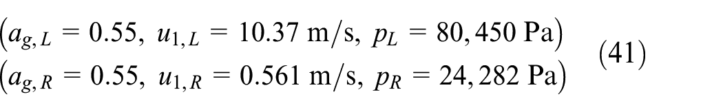
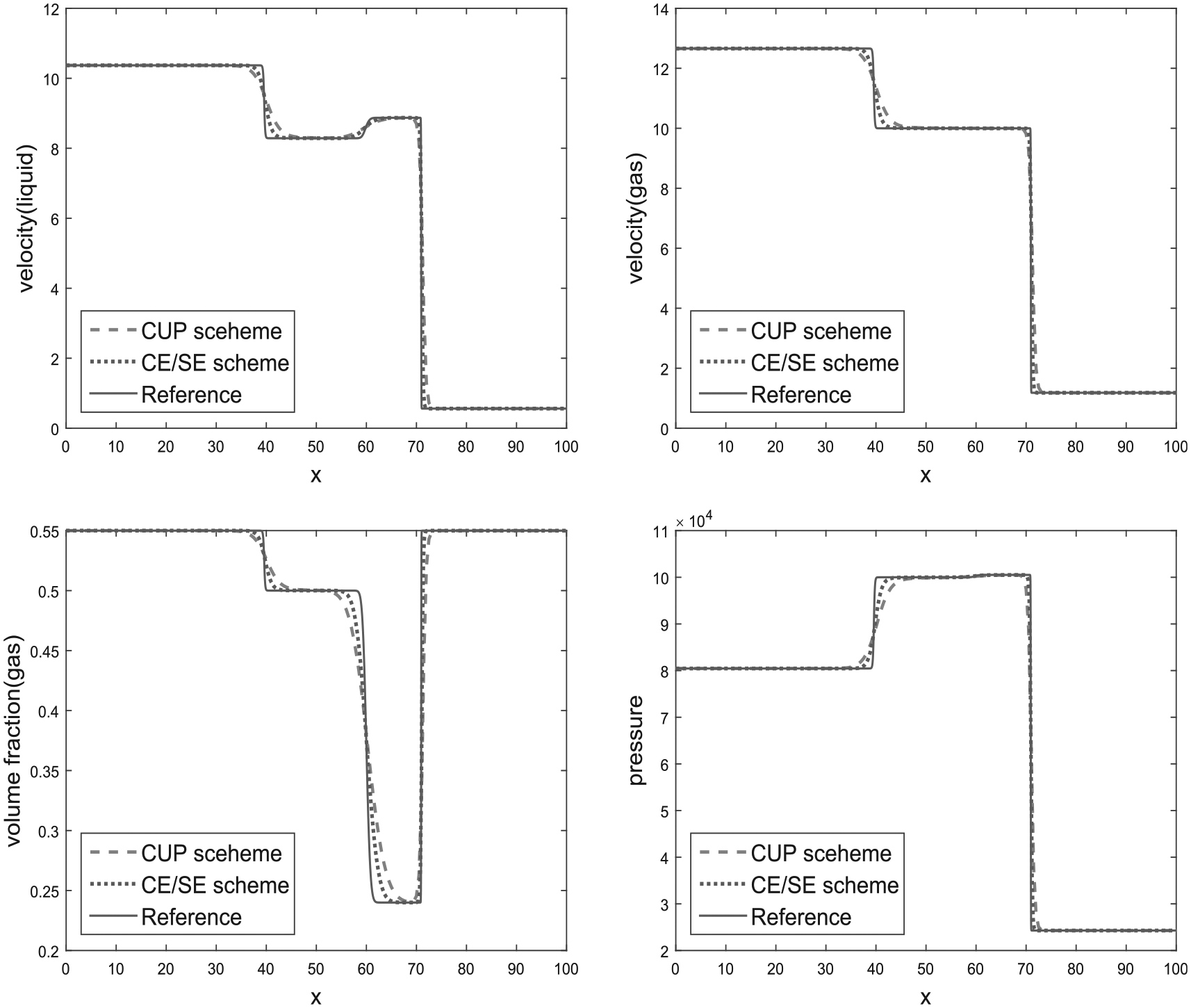
Test problem 4
The left and right states of this Riemann problem are

The solution composes of a left-going rarefaction wave, a contact discontinuity wave, and a right-going rarefaction wave, as shown in Figure 5. The solution profiles of phase velocities, volume fraction, and pressure are obtained from CE/SE and modified CUP schemes at time

Numerical results of shock tube problem by CE/SE and CUP schemes at
The last two problems were also considered in Fjelde and Karlsen.
4
These test problems are considered the hardest for the numerical schemes. In these test problems, the source term
Test problem 5
The first

Numerical results of pressure pulse and liquid velocity at different times by CE/SE and CUP schemes.
Test problem 6
In this test problem, the pipe is initially filled with stagnant liquid. By injecting liquid and gas at the inlet, the mass flow rate of liquid as well as gas increased to
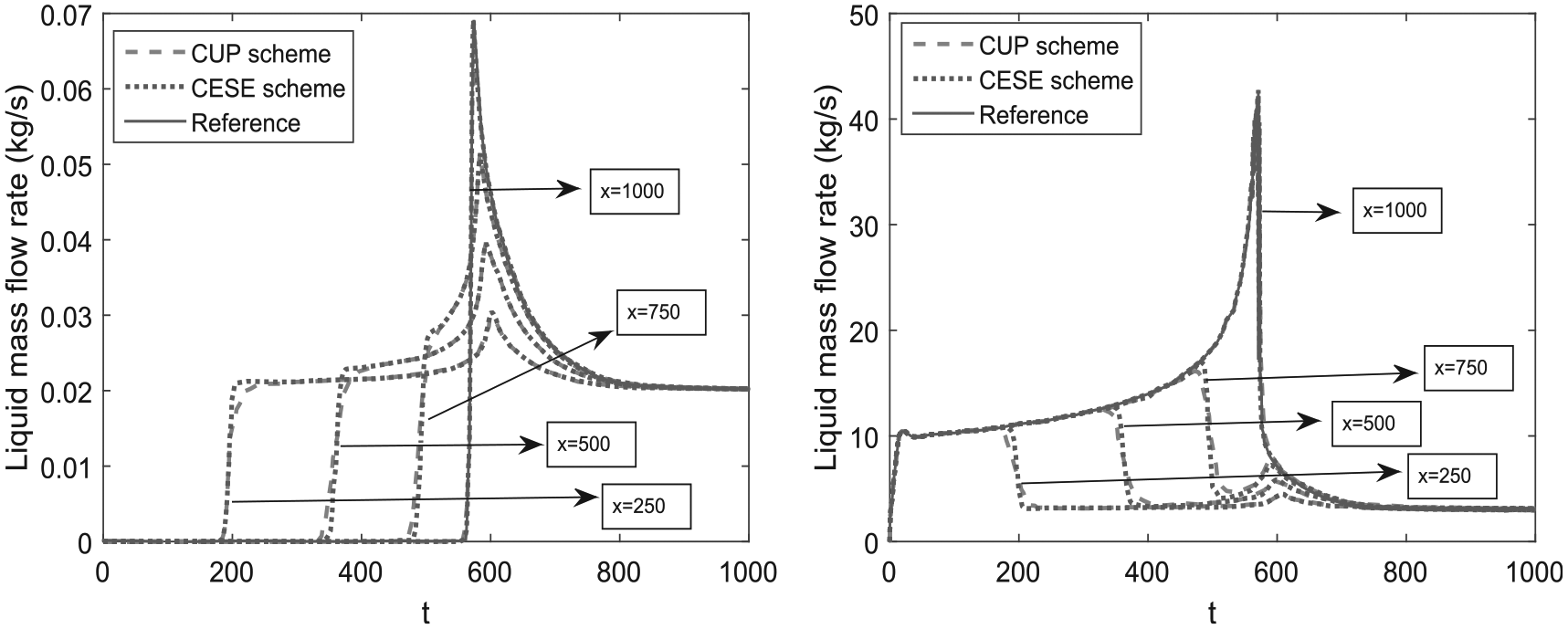
Numerical results at different positions by CE/SE and CUP schemes.
The gas and liquid passing through the horizontal pipe experience a decreasing pressure due to the frictional forces. As a consequence, the gas will expand, resulting in increased gas mass flow rates and the movement of liquid with larger velocity in front of the gas. Figure 7 shows that the liquid mass flow rate rises until the gas increases and decreases rapidly after passing the gas, while the rate of gas mass increases immediately when the gas arrives. The gas and liquid mass flow rates form sharp peaks at
Conclusion
In this article, the CE/SE scheme was extended to obtain the numerical solutions of the considered drift-flux model. The suggested numerical technique was capable to capture the volume-fraction discontinues without producing the oscillations. For comparison and validation, the modified CUP was also applied to solve the same drift-flux model. The number of test problems was considered. The numerical solutions obtained by CE/SE scheme verified the robustness, accuracy, and high resolutions for sharp discontinuities. A good agreement was found between the numerical solutions of both types of techniques, but CE/SE scheme has captured the strong shock waves and contact discontinuities more accurately and efficiently.
Footnotes
Handling Editor: James Baldwin
Declaration of conflicting interests
The author(s) declared no potential conflicts of interest with respect to the research, authorship, and/or publication of this article.
Funding
The author(s) received no financial support for the research, authorship, and/or publication of this article.