
Abstract
Model-based responses rarely coincide with the actual responses owing to modeling and measurement errors, deterioration of structural performance, and presence of damages in the structure. The parameter matrices should be updated for successful subsequent analysis and design efforts. This study derives the mathematical forms of variations in the parameter matrices between the actual system and the analytical model. A method using the least-squares principle constrained by the measured modal data is presented. The method is directly derived by minimizing the performance indices expressed by the norm of the variation in the parameter matrices between the actual system and the analytical model. The proposed update methods predict the updated parameter matrices depending on the prescribed weighting matrices and detect damages from the predicted parameter matrix variations. Examples compare the methods depending on the established weighting matrices, the number of measurement data sets of the first modal data only and the lowest two modal data. This study also investigates the effect of external noise contained in the measured data.
Introduction
It is difficult to accurately describe the responses of an actual system using the structural model established at the design stage because of inaccurate constructions, inhomogeneous properties of the structural materials, environmental effects, and measurement errors. The inaccurate utilization of the parameter matrices, such as the mass and stiffness matrices of the dynamic system, leads to the responses being deviated from the initial responses. Such inaccuracies should be minimized for successful subsequent analysis and design.
Numerous studies pertaining to the handling of updated parameter matrices of a finite-element model using only measured data have been reported. The updated parameter matrices can also be utilized as evidence to determine the defect in dynamic systems. The parameter matrices are primarily corrected using the least-squares methods and the parameter sensitivity methods.
The parameter-updating methods are used for obtaining responses that are as close as possible to the experimental and actual responses. Wang et al. 1 compared the modal parameter–based and flexibility-based damage-identification methods by optimizing the objective functions of a weighted function of the frequency and mode shapes and modal flexibility residue, respectively. Schommer et al. 2 discussed the difference between stiffness and the flexibility matrix for structural health monitoring based on vibrational measurements. They found that the flexibility-based quantification and localization of damage are more difficult. Lekidis et al. 3 developed a finite-element model-updating method based on an incomplete set of modal frequencies and mode shapes. Başağa et al. 4 proposed an updating algorithm for the uncertain parameters for each mode by minimizing the difference between the analytical and experimental natural frequencies. Fuentes 5 introduced and compared analytical methods that combine the mode-shaped expansion methods and the update methods of the stiffness parameters. Rim et al. 6 predicted the updated forms of the parameter matrices based on the estimated mode shape data. Chen and Tee 7 presented the optimized solutions in the least squares from the difference in the structural parameters between the finite-element model and the associated tested structure. Sheinman 8 provided an analytical algorithm for damage detection and for updating parameter matrices using the minimum static and/or dynamic measured modes and preserved the connectivity. Pokharkar and Shrikhande 9 provided an updated time-domain least-squares method to identify the structural stiffness and mass matrices using the condensed model. Sung et al. 10 presented a damage-detection approach for cantilever beam-type structures using the deflection estimated by the modal flexibility matrix. Rainieri et al. 11 provided dynamic identification techniques for the non-destructive evaluation of heritage structures.
Katebi et al. 12 obtained a damage-identification method using changes in the sensitivity matrix and the measured flexibility data. Chen and Nagarajaiah 13 derived the structural parameter optimization method by minimizing the Frobenius norm of the change in the flexibility matrix and the Gauss–Newton method for solving the optimization problem. Li et al. 14 presented a method for detecting reduction in the stiffness parameters of a structure using a generalized flexibility matrix and changes in natural frequencies. Yang and Sun 15 proposed a damage-detection method based on the best achievable flexibility change to localize and quantify damages. Cao et al. 16 proposed a model-updating method based on the residual flexibility mixed-boundary substructure method. Using the linear relationship between the flexibility matrix element and the structural parameter, Yang et al. 17 introduced the modal parameter and damage coefficient and provided a flexibility-based method for identifying the location and extent of the damage. Lacidogna et al. 18 investigated the damage propagation process using the acoustic emission technique and the extraction of resonance frequencies. They also evaluated the damage mechanisms for the stress-dependent damage progress using the acoustic emission and dynamic identification techniques. 19
Existing modal identification methods require extensive interaction and computational efforts. There have been research efforts for automated modal identification and tracking procedure. Rainieri and Fabbrocino 20 presented a literature review on automated operational modal analysis and developed algorithm aiming at fully automated output-only modal identification. They also investigated the validity of the automated output-only modal parameter estimation algorithm. 21 Rainieri et al. 22 proposed the use of second-order blind identification to estimate modal property.
The dynamic systems can be modeled by a system of fractional differential equations (FDEs). Using the operational matrix for fractional integral operator based on Chebyshev polynomials, a system of linear algebraic equations is derived and the numerical approximation can be obtained by solving system of Mittag–Leffler non-singular FDEs. Efficient numerical methods to solve a system of Mittag–Leffler non-singular FDEs have been considered.23–28
This article presents the mathematical forms of the updated parameter matrices to satisfy the flexibility matrix and eigenfunction established by the measured modal data using the least-squares approach. The update method is straightforwardly derived by minimizing the objective functions to satisfy the measured modal data. The parameter matrices take different mathematical forms depending on the prescribed objective functions and the weighting matrices. The numerical examples exhibit that the stiffness matrix as the weighting matrix indicates more accurate damage information than the mass matrix despite the external noise. It is found that the sensitivity to external noise contained in the measured mode shape data disappears in the use of accumulated data through repeated numerical simulations. The resulting method can be extended for detecting damages using the finite-element method. Furthermore, the predicted parameter matrices compare the validity of the proposed methods depending on the measured number of lowest modal data sets.
The structure of this article is as follows: In section “Estimation of updated stiffness and mass matrices,” we derive the mathematical forms to update stiffness matrix as well as mass matrix, and the corresponding example is presented to illustrate the validity of the proposed methods and to compare the numerical results depending on the presumed weighting matrices. In section “Estimation of updated stiffness matrix,” the mathematical forms to correct stiffness matrix are provided under the assumption of constant mass matrix. A numerical example is presented to validate the derived methods. In section “Conclusion,” the results of this study are summarized.
Formulations and examples
Estimation of updated stiffness and mass matrices
The dynamic equation for an undamped dynamic system of free vibration with n degrees of freedom (DOFs) can be expressed by

where
The characteristic equation of the dynamic system may be written as

where


where the mode shape vectors are taken utilizing the mass normalization
Taking the lowest
where the matrix
The parameter matrices are derived by the least-squares method to minimize the performance index. In this study, the objective functions were utilized by combining the objective functions utilized by Berman and Nagy 30 and Caeser and Pete 31 as


where “^” indicates the analytical parameter matrices. It is shown that the analytical mass and stiffness matrices are utilized as the weighting matrices.
This study compares the mathematical forms to describe the updated stiffness and mass matrices depending on the selected performance indices. Four different cases that combine the performance indices in equation (6) for predicting the stiffness and mass matrices are considered; (a) Case 1: D3 +D4, (b) Case 2: D3 +D2, (c) Case 3: D1 +D2, (d) Case 4: D1 +D4. The updated parameter matrices are independently derived according to the weighting matrices in the performance index. The performance index corresponding to Case 1 can be written by

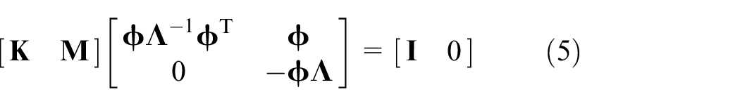
To utilize the performance index of equation (7) into equation (5), equation (5) is modified as

where

where “+” denotes the Moore–Penrose inverse, and
Inserting the condition to minimize equation (7) into equation (9) and solving the result with respect to the arbitrary matrix, we obtain

where

Post-multiplying both sides of equation (11) by
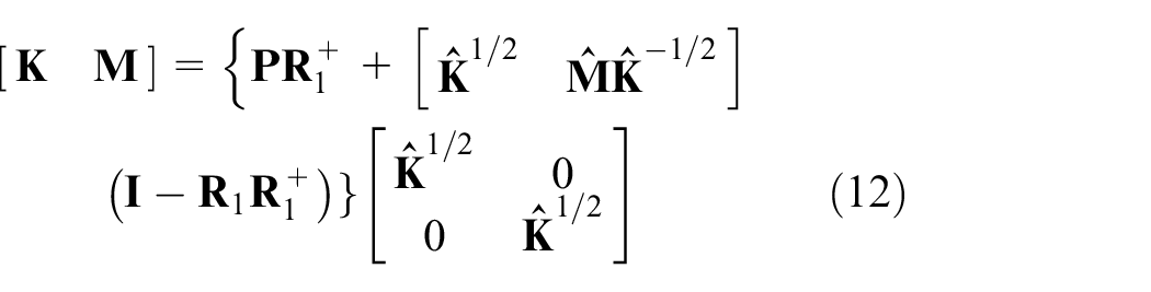
Equation (12) represents the mathematical forms of the parameter matrices that minimizes the performance index defined in equation (7). By the similar process as Case 1, the other cases can be similarly derived depending on the performance indices as
Case 2


Case 3


Case 4


Equations (12)–(15) represent the established performance indices and the corresponding mathematical forms to describe the updated parameter matrices. The parameter matrices take different forms depending on the weighting matrices. The numerical comparison is performed in the example.
Example 1
The correction methods of the parameter matrices proposed in this study are compared depending on the objective functions in the finite-element model of a fixed-end beam, as shown in Figure 1, whose applicability in the detection of damaged elements is examined. The beam length is 1 m, the length of each beam element is 20 mm, and the beam is modeled by 50 beam elements. The nodal points and elements are numbered in the figure. Each node has two DOFs of vertical displacement and slope, but the slope is neglected because it exhibits difficulty in collecting the rotational responses in the actual structure. The beam has an elastic modulus of  .
.
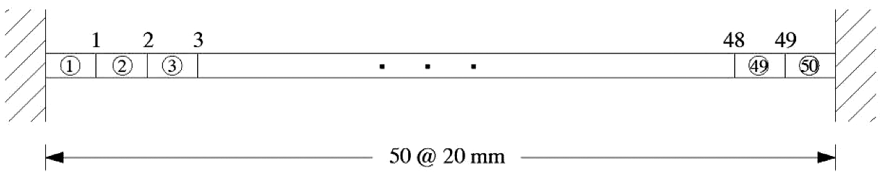
A fixed-end beam structure model.
The difference between the analytical and actual stiffness matrices at the damaged state is plotted in Figure 2. It is observed that, where the abrupt change in the parameter matrices is located at the damaged elements.
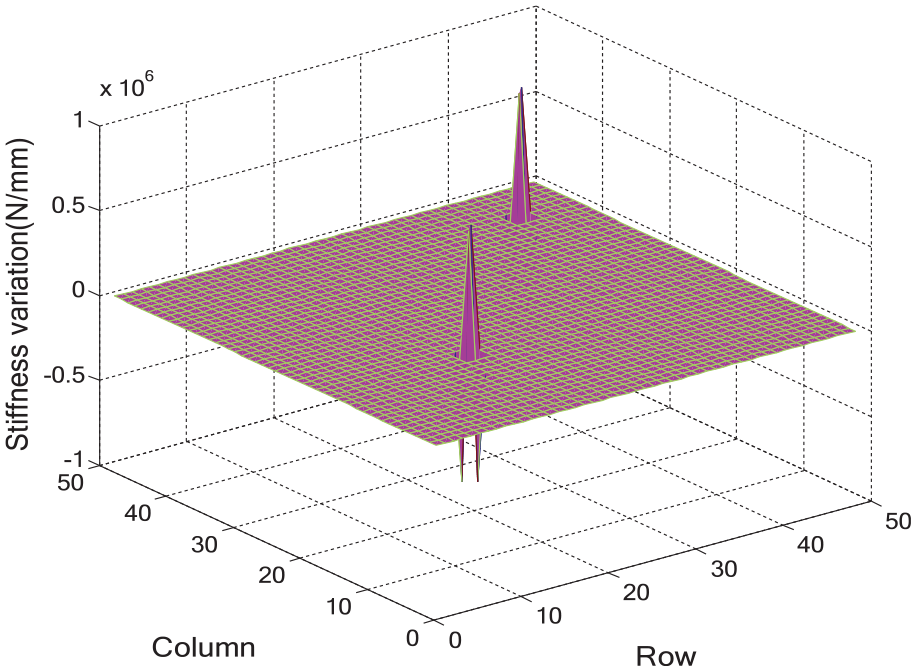
Variation between actual and analytical stiffness matrices.
The parameter matrices are updated using the noise-free first modal data only as the measurement data. The plots in Figure 3 represent the differences between the analytical and estimated parameter matrices. The proposed methods do not accurately describe the parameter matrices. The plots in Figure 3 compare the parameter matrices of the four cases estimated using the noise-free first modal data only. The variations in the stiffness and mass matrices exhibit different values depending on the weighting matrices. It is observed that the difference in the parameter matrices is decreased in using the analytical stiffness matrix as the weighting matrix rather than the analytical mass matrix, as shown in the updated stiffness and mass matrix plots in Case 1 (Cases 1-K and 1-M), updated stiffness matrix plot in Case 2 (Case 2-K), and updated stiffness matrix plot in Case 2 (Case 2-K). The damaged elements are located at the elements to exhibit the abrupt change in the parameter matrices. The updated stiffness and mass matrices exhibit significant differences when the analytical mass matrix is used as the weighting matrix, so the variation plots rarely provide the damage information, as listed in Figure 3.

Variations in parameter matrices estimated using noise-free first modal data only.
Figure 4 lists the differences between the parameter matrices predicted using the lowest two modal data sets as the measurement data; noise-free measurement data are assumed. The plots considering the analytical stiffness matrix as the weighting matrix show that the parameter matrices yield more accurate results with an increase in the number of mode shapes that participate in updating them. It is expected that the estimation of the updated parameter matrices gradually approaches the actual ones with an increase in the measured mode number.

Variations in parameter matrices estimated using two noise-free measured modal data.
Table 1 lists the suitability of the weighting matrix to update the parameter matrices synthesizing the results listed in Figures 3 and 4, where “○/A” and “X/B” indicate the suitability and unsuitability of matrices A and B as the weighting matrices, respectively. It is observed that the utilization of the stiffness matrix provides more reasonable results.
Comparison of the suitability of weighting matrices.

“○/A” and “X/B” indicate the suitability and unsuitability of the matrices A and B as the weighting matrices, respectively.
This study also investigates the effect of external noise contained in the measured mode shapes. The errors included in the measured data lead to some deviations from the analytical results. A simulated data set is established by adding a series of random numbers to represent errors in the calculated mode shape data. The ith measured mode shape vector

where
Figure 5 lists the variations in the stiffness and mass matrices estimated using the lowest two modal data sets contaminated by 2% noise level in equation (16), where “

Variations in parameter matrices estimated using the lowest two modal data contaminated by 2% noise: (a) Case 1-K, (b) Case 1-M, (c) Case 2–K, and (d) Case 4-M.
Figure 5 shows the variation matrix between the analytical and updated parameter matrices estimated using the lowest two modal data sets of 2% noise level. It displays the stiffness and mass curves corresponding to the diagonal elements in the parameter matrices and their curvature in Figure 5, respectively, using a central difference approximation
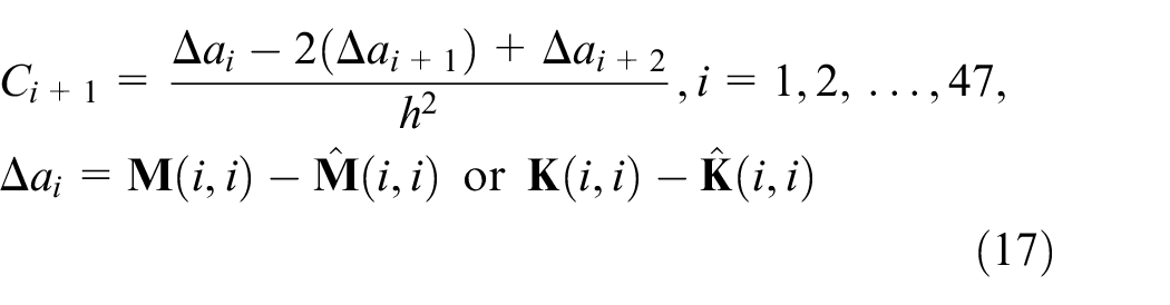
where
The effect of 2% noise level is investigated considering the cases listed in Table 1. The variation curves in the stiffness and mass matrices exhibit an abrupt change at the damaged elements in Figure 6(a), (c), (e), and (g). Similarly, the curvature curves in Figure 6(b), (d), (f), and (h) provide information on the damaged elements. A comparison of the variation curves indicates that the utilization of the updated stiffness matrix in Figure 5(a) and (e) provides more accurate damage information than the updated mass matrix in Figure 6(c) and (g) despite the external noise.

Diagonal elements in variation matrices between analytical and estimated parameters using 2% noise level and the first two modal data sets: (a) Case 1-K, (b) curvature of Case 1-K, (c) Case 1-M, (d) curvature of Case 1-M, (e) Case 2-K, (f) curvature of Case 2-K, (g) Case 4-M, and (h) curvature of Case 4-M.
Estimation of updated stiffness matrix
Assuming the invariant mass

where
The updated stiffness matrix

As indicated in the previous example, the analytical stiffness matrix
The constraint equation (18) is not related to the specific mode independently but is established by the modal data accumulated in the specific mth mode. Thus, the constraint interdependently affects the modal data within the mth mode. The stiffness variation matrix is derived by inserting the constraint condition of equation (18) into the performance index.
To insert the condition to minimize the performance index of equation (19), equation (18) is modified as

where
Solving equation (20) with respect to

where
Applying the minimization condition of equation (19) into equation (21), the arbitrary matrix

where

Post-multiplying both sides of equation (23) by
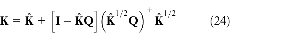
The second term on the right-hand side of equation (24) represents the variation in the stiffness matrix owing to the deterioration of structural performance, external noise, construction, and measurement errors. The modal data are related to the stiffness variation. The variable
Example 2
The second example considers damage detection using the stiffness variation alone. Assuming the invariant mass matrix, this example evaluates the numerical results of the updated methods by the lowest two modal data sets depending on the external noise. The measured modal data replaced by the numerically simulated data are utilized to estimate the stiffness matrix. The numerical experiments update the stiffness matrix using the lowest two modes (F-2 beam model). The responses of the F-2 beam model are constrained by the lowest two natural frequencies and the corresponding mode shapes.
The stiffness matrix of the F-2 beam model is updated by equation (24) and noise-free measurement modal data. Figure 7(a) shows the stiffness variation matrix before and after the damage occurrence. This shows that the abrupt change in the stiffness is limited to the damaged elements. The proposed approach does not yield accurate stiffness variations compared to the actual variations because the beam model is constrained by the lowest two modal data sets only. The abrupt variations are found at the damaged elements by the curve of the diagonal elements in the stiffness variation matrix and its curvature curve, as shown in Figure 7(b) and (c), respectively. As shown in the plots, the damage can be accurately detected by the stiffness variations in the case of noise-free measurement data.

Numerical results using noise-free measurement data: (a) stiffness variation matrix, (b) diagonal elements in the stiffness variation matrix and (c) curvature of diagonal elements.
The external noise contained in the measured mode shape data leads to the deviation in the actual stiffness as well as the actual modal data. Figure 8(a) shows the estimated stiffness variations including 2.0% noise, where the irregularity in the stiffness variations is observed unlike the noise-free case. The plots display the sensitivity to external noise. Figure 8(b) and (c) shows the numerical results using the lowest two modal data only contaminated by 2% noise level. It is expected that the damages are located in the neighborhood of element  , except for the actual damaged elements ⑱ and , as shown in Figure 8(b) and (c). This is caused by the external noise, and the inaccuracy of damage detection disappears in the use of accumulated data through repeated numerical simulations. It is found that the proposed method for updating the stiffness matrix can be utilized in detecting the damage despite the external noise.

Numerical results using 2% noise-contaminated measurement data: (a) stiffness variation matrix, (b) diagonal elements in the stiffness variation matrix, and (c) curvature of diagonal elements.
Conclusion
The dynamic responses of the analytical model do not coincide with the actual ones, and the dynamic parameter matrices should be corrected for subsequent analyses. This article proposes the mathematical forms for updating the stiffness and mass matrices. However, the method rarely provides accurate parameter matrices. It is shown that the parameter matrices are straightforwardly derived and take explicitly different forms depending on the weighting matrices in the objective functions. In comparing the variation curves to utilize the stiffness and mass matrices, it is observed that the stiffness matrix as the weighting matrix indicates more accurate damage information than the mass matrix despite the external noise. In addition, the method in section “Estimation of updated stiffness matrix” to update the stiffness matrix can only also be utilized in detecting the damage despite the external noise. It is not practical to collect the data of a full set of DOFs. More research on the update of parameter matrices is required because of using fewer measurement data than the system DOF.
Footnotes
Handling Editor: Dumitru Baleanu
Declaration of conflicting interests
The author(s) declared no potential conflicts of interest with respect to the research, authorship, and/or publication of this article.
Funding
The author(s) disclosed receipt of the following financial support for the research, authorship, and/or publication of this article: This research is supported by the Basic Science Research Program through the National Research Foundation of Korea (NRF) funded by the Ministry of Education (grant no. NRF-2016R1D1A1A09918011) and also by the 2018 Research Grant (PoINT) from Kangwon National University.