Regressor-free adaptive fuzzy force tracking control of redundant robot manipulator for task space

Abstract

In this study, an adaptive fuzzy force control of a redundant robot manipulator experiencing system uncertainties and operating in an unknown environment is proposed. This is important not only to provide additional control flexibility for complicated tasks but also to avoid the joint limit of a robot in implementing better dynamics and kinematics. The relation between the task and joint spaces is discussed to derive a dynamic model for force tracking controller design. To treat the system uncertainties, an adaptive fuzzy system approach is established to achieve the adaptive position and force controller design based on a regressor-free approach. Considering that the stiffness coefficient of the environment is assumed to be unknown, the gradient descent method is used to estimate this coefficient to achieve adaptive force tracking. A stability analysis of the closed-loop system and the corresponding update laws are given by the Lyapunov stability theorem. Finally, several apposite simulations using the KUKA lightweight robot are performed to validate our approach and demonstrate the performance and effectiveness of the proposed regressor-free adaptive fuzzy force controller.

Introduction

In recent years, industrial automatic manipulators are being widely used to reduce the burden of labor. Some robot manipulators can deal with free space motion and interaction with contact environments such as welding, polishing, and cutting. Many controller design methods have been proposed to solve the tracking control of robot manipulator.^1–5 One in the existing literature ⁵ has proposed a semi-global asymptotic stability analysis via Lyapunov theorem for a new proportional-integral-derivative (PID) controller based on the fuzzy system for tuning controller gains to improve the performance. Several articles have also introduced the adaptive controller for robot manipulator.^2,6–8 Usually, the end-effector of the robot manipulator not only implemented the tracking trajectory but also prevent the over crash on the contact environment. Therefore, force/position control and impedance control have been presented to deal with the external force control.^{2,3,6,7,9–11} This means that the adaptive force control is achieved by fine-tuning the desired trajectories. In this article, the results are extended to redundant robot manipulators that have to encounter in their task space system uncertainties and work in unknown environments (unknown stiffness coefficient). The redundant robot manipulators can provide additional control flexibility for complicated tasks and avoid the joint limit of a robot to implement better dynamics and kinematics.^12–14 As discussed above, the adaptive force control of redundant robot manipulator is less common; therefore, the results of adaptive fuzzy force control for redundant robot systems is introduced in this article.

The mapping of the joint space to the task space cannot clearly illustrate all the dynamic behavior in the redundancy case. Thus, the null space and the relation between the task and joint spaces are considered to derive the dynamic model of the redundant robot manipulator. In our investigation, the dynamic model of the redundant robot manipulator is assumed to be unknown or not exactly known.^12–17 Therefore, the fuzzy systems are utilized to be estimators for estimating the dynamic model. Based on the Lyapunov approach, the tracking control can be achieved by adaptive fuzzy control approach, that is, the tracking error will approach to zero when time is approaching infinity. Besides, for force control problem, the adaptive path planning is designed to solve force tracking when the stiffness of the contact material is unknown. The corresponding stiffness coefficient is estimated by gradient method and the convergence is also guaranteed by Lyapunov approach.

The rest of this research is organized as follows. In section “Dynamic model of redundant robot manipulator,” the dynamic model of the redundant robot manipulator with null space is introduced. Section “Regressor-free adaptive force controller design” introduces the regressor-free adaptive force control of redundant robot manipulator via the adaptive fuzzy scheme. In section “Simulation results,” the simulations of redundant robot manipulator are introduced to illustrate the effectiveness of our controller design. Finally, the conclusions are given.

Dynamic model of redundant robot manipulator

Because of the properties of redundancy, the mapping of joint space to the task space cannot clearly illustrate all the dynamic behavior. Therefore, the problem is transferred to the velocity and acceleration level using the pseudo-inverse of the Jacobian matrix of the manipulator. Here, we consider the null space and relation between the task and joint spaces to derive the dynamic model of the redundant robot manipulator. At first, the dynamic model of n degree of freedom (DOF) robot manipulator is

$$\mathbf{M}\left(\mathbf{q}\right)\stackrel{··}{\mathbf{q}}+\mathbf{C}(\mathbf{q},\stackrel{·}{\mathbf{q}})\stackrel{·}{\mathbf{q}}+\mathbf{g}\left(\mathbf{q}\right)+{\mathbf{\tau }}_{\mathrm{ext}}=\mathbf{\tau }$$

(1)

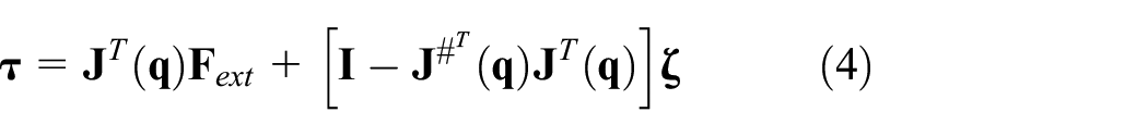
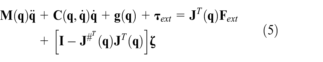
where $\mathbf{q},\stackrel{·}{\mathbf{q}},\stackrel{··}{\mathbf{q}}\in {\Re }^n$ are the joint position, velocity, and acceleration, respectively; $\mathbf{M}(\mathbf{q})\in {\Re }^{n\times n}$ is the symmetric bounded positive definite inertia matrix; $\mathbf{C}(\mathbf{q},\stackrel{·}{\mathbf{q}})\stackrel{·}{\mathbf{q}}\in {\Re }^n$ is the vector of centrifugal and Coriolis torque; $\mathbf{g}(\mathbf{q})\in {\Re }^n$ is gravitational torque; $\mathbf{\tau }\in {\Re }^n$ is control torque, and ${\mathbf{\tau }}_{\mathrm{ext}}\in {\Re }^m$ is external torque resulting from the interaction with the environment. The external torque can be directly measured by force sensor. Many literature works introduced the adaptive impedance control by the regressor property;^2,3,15 however, here a regressor-free adaptive approach for redundant robot manipulator with uncertainties and unknown environment parameters is introduced.

For the force tracking control problem, the control strategy for task space is intuitive and better than the result for joint space. We first discuss the relation between task and null spaces. $\mathbf{p}=[\begin{array}{cccccc}x\hfill & y\hfill & z\hfill & \varphi \hfill & \theta \hfill & \psi \hfill \end{array}{]}^T$ denotes the end-effector position and orientation. The relation between the joint and task velocities are given by the Jacobian matrix: $\mathbf{J}(\mathbf{q})\in {\Re }^{m\times n}$ ^4,13,16–18

$${\mathbf{p}}_r=\mathbf{J}\stackrel{·}{\mathbf{q}}$$

(2)

where ${\mathbf{p}}_r=[\stackrel{·}{x}\stackrel{·}{y}\stackrel{·}{z}{\omega }_x{\omega }_y{\omega }_z{]}^T$ . In the redundant case of n > m, r = n − m is called the degree of redundancy; a set of coordinates cannot clearly describe the end-effector position and orientation and completely specify the configuration of the redundant robot manipulator, however, the behavior of end-effector should be obtained. In addition, when J⁻¹ does not exist, the pseudo-inverse ${\mathbf{J}}^{+}={\mathbf{J}}^T(\mathbf{J}{\mathbf{J}}^T{)}^{-1}$ is used.

Considering the results obtained using the Jacobian matrix,^4,13,16–18 it is desirable to find a solution based on an appropriate weighting (usually the inertia matrix M) of the components in many applications. Therefore, we chose the weighted pseudo-inverse ${\mathbf{J}}^{\#}\in {\Re }^{n\times m}$ ,^3,6,9,14,19 that is, $\mathbf{J}{\mathbf{J}}^{\#}=\mathbf{I}$ . When the end-effector of the redundant robot manipulator comes into contact with the external environment, the interaction force is obtained. Thus, we define the external interaction force ${\mathbf{F}}_{\mathrm{ext}}\in {\Re }^m$ and

$${\mathbf{\tau }}_{\mathrm{ext}}={\mathbf{J}}^T\left(\mathbf{q}\right){\mathbf{F}}_{\mathrm{ext}}$$

(3)

However, the decomposed analysis shows that there is an infinity of elementary displacements without altering the configuration of the end-effector and that it is also affected by the null space.^18,19 For the general form, we can design

$$\mathbf{\tau }={\mathbf{J}}^T\left(\mathbf{q}\right){\mathbf{F}}_{\mathrm{ext}}+[\mathbf{I}-{\mathbf{J}}^{{\mathrm{\#}}^T}\left(\mathbf{q}\right){\mathbf{J}}^T\left(\mathbf{q}\right)]\mathbf{\zeta }$$

(4)

where $\mathbf{\zeta }$ is an arbitrary generalized joint torque vector projected in the null space of ${\mathbf{J}}^{+}$ . Thus

$$\begin{array}{cc}\multicolumn{1}{c}{\mathbf{M}\left(\mathbf{q}\right)\stackrel{··}{\mathbf{q}}}& +\mathbf{C}(\mathbf{q},\stackrel{·}{\mathbf{q}})\stackrel{·}{\mathbf{q}}+\mathbf{g}\left(\mathbf{q}\right)+{\mathbf{\tau }}_{\mathrm{ext}}={\mathbf{J}}^T\left(\mathbf{q}\right){\mathbf{F}}_{\mathrm{ext}}\hfill \\ \multicolumn{1}{c}{}& +[\mathbf{I}-{\mathbf{J}}^{{\mathrm{\#}}^T}\left(\mathbf{q}\right){\mathbf{J}}^T\left(\mathbf{q}\right)]\mathbf{\zeta }\hfill \end{array}$$

(5)

Multiplying $\mathbf{J}{\mathbf{M}}^{-1}$ and defining ${\stackrel{··}{\mathbf{p}}}_r=\stackrel{.}{\mathbf{J}}\stackrel{.}{\mathbf{q}}+\mathbf{J}\stackrel{··}{\mathbf{q}}$ , we have

$$\begin{array}{c}{\stackrel{·}{\mathbf{p}}}_r+(\mathbf{J}{\mathbf{M}}^{-1}\mathbf{C}\stackrel{·}{\mathbf{q}}-\stackrel{·}{\mathbf{J}}\stackrel{·}{\mathbf{q}})+\mathbf{J}{\mathbf{M}}^{-1}\mathbf{g}+{\mathbf{\tau }}_{\mathrm{ext}}\hfill \\ =\left(\mathbf{J}{\mathbf{M}}^{-1}{\mathbf{J}}^T\right){\mathbf{F}}_{\mathrm{ext}}+\mathbf{J}{\mathbf{M}}^{-1}(\mathbf{I}-{\mathbf{J}}^{{\mathrm{\#}}^T}{\mathbf{J}}^T)\mathbf{\zeta }\hfill \end{array}$$

(6)

This means that the joint torque of null space will not generate any command acceleration, that is, $[\mathbf{J}{\mathbf{M}}^{-1}-(\mathbf{J}{\mathbf{M}}^{-1}{\mathbf{J}}^T){\mathbf{J}}^{{\mathrm{\#}}^T}]\mathbf{\zeta }=0$ and the dynamic consistency matrix ${\mathbf{J}}^{{\#}^T}=\mathbf{J}{\mathbf{M}}^{-1}(\mathbf{J}{\mathbf{M}}^{-1}{\mathbf{J}}^T{)}^{-1}$ is obtained. For the general solution, the joint velocity is

$$\stackrel{·}{\mathbf{q}}={\mathbf{J}}^{\#}{\mathbf{p}}_r+(\mathbf{I}-{\mathbf{J}}^{\#}\mathbf{J}){\stackrel{·}{\mathbf{q}}}_N$$

(7)

where ${\mathbf{J}}^{\#}={\mathbf{M}}^{-1}{\mathbf{J}}^T(\mathbf{J}{\mathbf{M}}^{-1}{\mathbf{J}}^T{)}^{-1}$ , ${\mathbf{N}}^{\#}=\mathbf{I}-{\mathbf{J}}^{\#}\mathbf{J}$ , ${\mathbf{N}}^{\#}\in {\Re }^{n\times n}$ is the matrix which projects $\stackrel{·}{\mathbf{q}}$ to the null space of J, that is, $\mathbf{J}{\mathbf{N}}^{\#}\stackrel{·}{\mathbf{q}}=0$ , ${\stackrel{·}{\mathbf{q}}}_N\in {\Re }^{n\times 1}$ is the joint velocity vector. From (7), we obtain

$$\stackrel{·}{\mathbf{q}}={\stackrel{·}{\mathbf{q}}}_p+{\stackrel{·}{\mathbf{q}}}_h={\mathbf{J}}^{\#}{\mathbf{p}}_r+(\mathbf{I}-{\mathbf{J}}^{\#}\mathbf{J}){\stackrel{·}{\mathbf{q}}}_N$$

(8)

where ${\stackrel{·}{\mathbf{q}}}_p$ is related with the task space motion and ${\stackrel{·}{\mathbf{q}}}_h$ is the projected velocity vector in the null space related to the null space motion. However, ${\stackrel{·}{\mathbf{q}}}_h$ is not a minimal set to specify the null space motion. Therefore, the r-dimensional vectors are necessary to specify the null space of J. ${\stackrel{·}{\mathbf{q}}}_p$ is in the row space of Jacobian matrix, $\Re ({\mathbf{J}}^T)$ , and ${\stackrel{·}{\mathbf{q}}}_h$ is in the null space of Jacobian matrix N (J). Because $\Re ({\mathbf{J}}^T)$ and N(J) are orthogonal, ${\stackrel{·}{\mathbf{q}}}_p$ and ${\stackrel{·}{\mathbf{q}}}_h$ are also orthogonal. By the properties of linear algebra, the general solution ${\stackrel{·}{\mathbf{q}}}_h$ constructs the null space of the Jacobian matrices. We define $\mathbf{Z}(\mathbf{q})\in {\Re }^{n\times r}$ satisfying the condition $\mathbf{J}{\mathbf{N}}^{\mathrm{\#}}\stackrel{·}{\mathbf{q}}=0$ ; therefore, the joint motion of null space will not affect the end-effector motion (called self-motion). In addition, $(\mathbf{I}-{\mathbf{J}}^{\#}\mathbf{J}){\stackrel{·}{\mathbf{q}}}_N$ is the projection matrix of null space, that is, the realization of the second task can be achieved by choosing different velocities of the null space. Thus, system (2) is

$$\begin{array}{cc}\multicolumn{1}{c}{\stackrel{·}{\mathbf{q}}}& ={\mathbf{J}}_E^{-1}\left(\mathbf{q}\right)\left[\begin{array}{c}{\mathbf{p}}_r\hfill \\ \multicolumn{1}{c}{\mathbf{v}}\end{array}\right]\mathbf{=}\left[\begin{array}{cc}{\mathbf{J}}^{\#}\left(\mathbf{q}\right)\hfill & \mathbf{Z}\left(\mathbf{q}\right)\hfill \end{array}\right]\left[\begin{array}{c}{\mathbf{p}}_r\hfill \\ \multicolumn{1}{c}{\mathbf{v}}\end{array}\right]\hfill \\ \multicolumn{1}{c}{}& ={\mathbf{J}}^{\#}\left(\mathbf{q}\right){\mathbf{p}}_r+\mathbf{Z}\left(\mathbf{q}\right)\mathbf{v}\hfill \end{array}$$

(9)

and

$$\stackrel{··}{\mathbf{q}}={\stackrel{·}{\mathbf{J}}}^{\#}\left(\mathbf{q}\right){\mathbf{p}}_r\mathbf{+}{\mathbf{J}}^{\#}\left(\mathbf{q}\right){\stackrel{·}{\mathbf{p}}}_r+\stackrel{·}{\mathbf{Z}}\left(\mathbf{q}\right)\mathbf{v}\mathbf{+}\mathbf{Z}\left(\mathbf{q}\right)\stackrel{·}{\mathbf{v}}$$

(10)

Systems (9) and (10) are used to derive the dynamic model of the task and null spaces. System (1) is multiplied by ${\mathbf{J}}_E^{-T}(\mathbf{q})$ and combining the task and null spaces as

$${\mathbf{J}}_E^{-T}\mathbf{M}\stackrel{··}{\mathbf{q}}+{\mathbf{J}}_E^{-T}\mathbf{C}\stackrel{·}{\mathbf{q}}+{\mathbf{J}}_E^{-T}\mathbf{g}+{\mathbf{J}}_E^{-T}{\mathbf{\tau }}_{\mathrm{ext}}={\mathbf{J}}_E^{-T}\mathbf{\tau }$$

(11)

Substituting equations (9) and (10) into equation (11), we have

$$\begin{array}{c}{\mathbf{J}}_E^{-T}\mathbf{M}({\mathbf{J}}^{\mathbf{\#}}{\stackrel{·}{\mathbf{p}}}_r+\mathbf{Z}\stackrel{·}{\mathbf{v}})+{\mathbf{J}}_E^{-T}\mathbf{M}({\stackrel{·}{\mathbf{J}}}^{\mathbf{\#}}{\mathbf{p}}_r+\stackrel{·}{\mathbf{Z}}\mathbf{v})\hfill \\ +{\mathbf{J}}_E^{-T}\mathbf{C}({\mathbf{J}}^{\mathbf{\#}}{\mathbf{p}}_r+\mathbf{Zv})+{\mathbf{J}}_E^{-T}\mathbf{g}+{\mathbf{J}}_E^{-T}{\mathbf{\tau }}_{\mathrm{ext}}={\mathbf{J}}_E^{-T}\mathbf{\tau }\hfill \end{array}$$

(12)

Subsequently, system (1) can be transferred to the task and null spaces as

$$\begin{array}{c}\left[\begin{array}{cc}{\mathbf{A}}_t\hfill & 0\hfill \\ \multicolumn{1}{c}{0}& {\mathbf{A}}_{\nu }\hfill \end{array}\right]\left[\begin{array}{c}\stackrel{··}{\mathbf{p}}\hfill \\ \multicolumn{1}{c}{\stackrel{·}{\mathbf{v}}}\end{array}\right]+\left[\begin{array}{cc}{\mathbf{B}}_{\mathrm{tx}}\hfill & {\mathbf{B}}_{x\nu }\hfill \\ \multicolumn{1}{c}{{\mathbf{B}}_{\mathrm{tv}}}& {\mathbf{B}}_{\nu }\hfill \end{array}\right]\left[\begin{array}{c}\stackrel{·}{\mathbf{p}}\hfill \\ \multicolumn{1}{c}{\mathbf{v}}\end{array}\right]\hfill \\ +\left[\begin{array}{c}{\mathbf{G}}_x\hfill \\ \multicolumn{1}{c}{{\mathbf{G}}_v}\end{array}\right]+\left[\begin{array}{c}{\mathbf{F}}_{\mathrm{ext}}\hfill \\ \multicolumn{1}{c}{0}\end{array}\right]=\left[\begin{array}{c}{\mathbf{F}}_x\hfill \\ \multicolumn{1}{c}{{\mathbf{F}}_n}\end{array}\right]\hfill \end{array}$$

(13)

where ${\mathbf{A}}_t={\mathbf{A}}_x{\mathbf{R}}_E$ , ${\mathbf{B}}_{\mathrm{tx}}={\mathbf{A}}_x{\stackrel{·}{\mathbf{R}}}_E+{\mathbf{B}}_x{\mathbf{R}}_E$ , and ${\mathbf{G}}_x={\mathbf{J}}^{{\mathrm{\#}}^T}\mathbf{g}$ are the system parameters of task space model and ${\mathbf{B}}_{t\nu }={\mathbf{B}}_{\nu x}{\mathbf{R}}_E$ and ${\mathbf{G}}_v={\mathbf{Z}}^T\mathbf{g}$ are the system parameters of the null space model; F _x and F _n are control inputs of task and null spaces, respectively. As previous works,^2,6,7 we consider the system with uncertainties, therefore, the dynamic model matrices A _t , B _tx , B _tv , G _x , and G _v are not exactly known. Herein, we estimate them using established fuzzy systems denoting them ${\hat{\mathbf{A}}}_t$ , ${\hat{\mathbf{B}}}_{\mathrm{tx}}$ , ${\hat{\mathbf{B}}}_{\mathrm{tv}}$ , ${\hat{\mathbf{G}}}_x$ , and ${\hat{\mathbf{G}}}_v$ .

In this article, we assume that the task space and null space dynamic models of the redundant robot manipulator are complicated and unknown. In order to solve it, we develop an adaptive fuzzy control scheme to treat it, that is, fuzzy systems are established to estimate the dynamic model of the redundant robot manipulator and design the adaptive force controller such that the end-effector can track our desired trajectory in the task space and achieve the desired force for contact space even if the dynamic model is uncertain and the system is operated in an unknown environment.

Regressor-free adaptive force controller design

This section introduces the proposed adaptive force controller design using the fuzzy systems. The proposed approach is divided into two steps: the first one is adaptive tracking controller design for uncertain robot systems and the second is adaptive force control by desired position adaption.

Fuzzy systems

As discussed above, the unknown models of redundant robot manipulator are estimated by adaptive fuzzy systems. Here, the utilized fuzzy system is implemented by singleton fuzzifier, product inference, centroid defuzzifier, and Gaussian membership functions.^20,21 The jth fuzzy rule for estimator is

$$\mathrm{Rule}j:\mathrm{IF}{x}_i\mathrm{is}{A}_{\mathrm{ij}}\mathrm{and}\dots \mathrm{and}{x}_n\mathrm{is}{A}_{\mathrm{nj}},\mathrm{THEN}y\mathrm{is}{\omega }_j$$

(14)

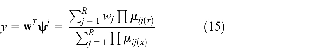
where x_i is the input variable of fuzzy system, A_ij is the fuzzy term set represented by Gaussian function, and ${\omega }_j$ is the consequent part for output y. Therefore, the fuzzy system’s output is

$$y={\mathbf{w}}^T{\mathbf{ѱ}}^j=\frac{\sum _{j=1}^R{w}_j\Pi {\mu }_{\mathrm{ij}\left(x\right)}}{\sum _{j=1}^R\Pi {\mu }_{\mathrm{ij}\left(x\right)}}$$

(15)

where $\mathbf{w}=[\begin{array}{cccc}{w}_1\hfill & w_2\hfill & \cdots \hfill & w_R\hfill \end{array}{]}^T$ is the weighting vector (adjustable parameters), R is the rule number and µ_ij(x) are the Gaussian membership functions of x associated with the corresponding fuzzy rule. According to the literature,^7,20 the fuzzy system shown in equation (15) has the property of universal approximation, that is, it has the ability to approximate any continuous function.

Adaptive tracking controller design

As explained above, we assume that the dynamic model matrices A _t , B _tx , B _tv , G _x , and G _v are not exactly known and are estimated using established fuzzy systems denoting them ${\hat{\mathbf{A}}}_t$ , ${\hat{\mathbf{B}}}_{\mathrm{tx}}$ , ${\hat{\mathbf{B}}}_{\mathrm{tv}}$ , ${\hat{\mathbf{G}}}_x$ , and ${\hat{\mathbf{G}}}_v$ . They are approximated by fuzzy systems and expressed in the form of equation (15), that is, ${\hat{\mathbf{A}}}_t={\hat{\mathbf{w}}}_{A_t}{\mathbf{ѱ}}_{A_t}$ , ${\hat{\mathbf{B}}}_{\mathrm{tx}}={\hat{\mathbf{w}}}_{B_{\mathrm{tx}}}{\mathbf{ѱ}}_{B_{\mathrm{tx}}}$ , ${\hat{\mathbf{B}}}_{\mathrm{tv}}={\hat{\mathbf{w}}}_{B_{\mathrm{tv}}}{\mathbf{ѱ}}_{B_{\mathrm{tv}}}$ , and ${\hat{\mathbf{G}}}_x={\hat{\mathbf{w}}}_{G_x}{\mathbf{ѱ}}_{G_x}$ . There exists optimal weighting vectors such that ${\mathbf{A}}_t={\mathbf{w}}_{A_t}^{*}{\mathbf{ѱ}}_{A_t}+{\mathbf{\epsilon }}_{A_t}$ , ${\mathbf{B}}_{\mathrm{tx}}={\mathbf{w}}_{B_{\mathrm{tx}}}^{*}{\mathbf{ѱ}}_{B_{\mathrm{tx}}}+{\mathbf{\epsilon }}_{B_{\mathrm{tx}}}$ , ${\mathbf{B}}_{\mathrm{tv}}={\mathbf{w}}_{B_{\mathrm{tv}}}^{*}{\mathbf{ѱ}}_{B_{\mathrm{tv}}}+{\mathbf{\epsilon }}_{B_{\mathrm{tv}}}$ , ${\mathbf{G}}_x={\mathbf{w}}_{G_x}^{*}{\mathbf{ѱ}}_{G_x}+{\mathbf{\epsilon }}_{G_x}$ , and ${\mathbf{G}}_v={\mathbf{w}}_{G_v}^{*}{\mathbf{ѱ}}_{G_v}+{\mathbf{\epsilon }}_{G_v}$ ; where, ${\mathbf{w}}_{A_t}^{*}\in {\Re }^{m^{2}R}$ , ${\mathbf{w}}_{B_{\mathrm{tx}}}^{*}\in {\Re }^{m^{2}R}$ , ${\mathbf{w}}_{B_{\mathrm{tv}}}^{*}\in {\Re }^R$ , ${\mathbf{w}}_{G_x}^{*}\in {\Re }^{\mathrm{mR}}$ , and ${\mathbf{w}}_{G_v}^{*}\in {\Re }^R$ are the optimal weighting matrices; ${\mathbf{ѱ}}_{A_t}\in {\Re }^{m^{2}R}$ , ${\mathbf{ѱ}}_{B_{\mathrm{tx}}}\in {\Re }^{m^{2}R}$ , ${\mathbf{ѱ}}_{B_{\mathrm{tv}}}\in {\Re }^R$ , ${\mathbf{ѱ}}_{G_x}\in {\Re }^{\mathrm{mR}}$ , and ${\mathbf{ѱ}}_{G_v}\in {\Re }^R$ are the firing strengths of the corresponding rules; and ${\mathbf{\epsilon }}_{A_t}$ , ${\mathbf{\epsilon }}_{B_{\mathrm{tx}}}$ , ${\mathbf{\epsilon }}_{B_{\mathrm{tv}}}$ , ${\mathbf{\epsilon }}_{G_x}$ , and ${\mathbf{\epsilon }}_{G_v}$ are the bounded approximation errors.

Let $\mathbf{e}=x-x_d$ and $\mathbf{s}=\stackrel{·}{\mathbf{e}}+\mathbf{ke}$ where $k\in {\Re }^{n\times n}$ is positive definite and diagonal.

Thus, we are ready to introduce the adaptive fuzzy controller as following.

Theorem 1

Considering the redundant robot manipulator of equation (13) with the adaptive control scheme shown in Figure 1 (red dashed block), the adaptive tracking controllers for the task and null spaces are

$$\begin{array}{c}{\mathbf{F}}_x={\hat{\mathbf{A}}}_t({\stackrel{··}{\mathbf{x}}}_d-\mathbf{k}\stackrel{·}{\mathbf{e}})+{\hat{\mathbf{B}}}_{\mathrm{tx}}({\stackrel{·}{\mathbf{x}}}_d-\mathbf{ke})+{\hat{\mathbf{G}}}_x-{\mathbf{k}}_d\mathbf{s}+{{\mathbf{F}}_{x\mathrm{\_}}}_{\mathrm{robust}}\hfill \\ {\mathbf{F}}_n={\hat{\mathbf{B}}}_{\mathrm{tv}}({\stackrel{·}{\mathbf{x}}}_d-\mathbf{ke})+{\hat{\mathbf{G}}}_v-{\mathbf{k}}_{n}v+{{\mathbf{F}}_{n\mathrm{\_}}}_{\mathrm{robust}}\hfill \end{array}$$

(16)

where k _d and k _n are positive definite constant matrices and F _{x_robust} and F _{n_robust} are robust controllers for task and null spaces, respectively. They are designed as

$$\begin{array}{cc}\multicolumn{1}{c}{{{\mathbf{F}}_{x\_}}_{\mathrm{robust}}}& =-{\stackrel{·}{\hat{\delta }}}_{A_t}\mathrm{sgn}(\mathbf{s})({\stackrel{··}{\mathbf{x}}}_d-\mathbf{k}\stackrel{·}{\mathbf{e}})\hfill \\ \multicolumn{1}{c}{}& -{\stackrel{·}{\hat{\delta }}}_{B_{\mathrm{tx}}}\mathrm{sgn}(\mathbf{s})({\stackrel{·}{\mathbf{x}}}_d-\mathbf{ke})-{\stackrel{·}{\hat{\delta }}}_{G_x}\mathrm{sgn}(\mathbf{s})\hfill \\ \multicolumn{1}{c}{{{\mathbf{F}}_{n\_}}_{\mathrm{robust}}}& =-{\stackrel{·}{\hat{\delta }}}_{B_{\mathrm{tv}}}\mathrm{sgn}(\mathbf{s})({\stackrel{·}{\mathbf{x}}}_d-\mathbf{ke})-{\stackrel{·}{\hat{\delta }}}_{G_v}\mathrm{sgn}(\mathbf{s})\hfill \end{array}$$

(17)

with the following update laws

$${\stackrel{·}{\hat{\delta }}}_{A_t}=-{\gamma }_{A_t}\mathrm{sgn}\left(\mathbf{s}\right)({\stackrel{··}{\mathbf{x}}}_d-\mathbf{k}\stackrel{·}{\mathbf{e}})$$

(18a)

$${\stackrel{·}{\hat{\delta }}}_{B_{\mathrm{tx}}}=-{\gamma }_{B_{\mathrm{tx}}}\mathrm{sgn}\left(\mathbf{s}\right)({\stackrel{·}{\mathbf{x}}}_d-\mathbf{ke})$$

(18b)

$${\stackrel{·}{\hat{\delta }}}_{B_{\mathrm{tv}}}=-{\gamma }_{B_{\mathrm{tv}}}\mathrm{sgn}\left(\mathbf{s}\right)({\stackrel{·}{\mathbf{x}}}_d-\mathbf{ke})$$

(18c)

$${\stackrel{·}{\hat{\delta }}}_{G_x}=-{\gamma }_{G_x}\mathrm{sgn}\left(\mathbf{s}\right)$$

(18d)

$${\stackrel{·}{\hat{\delta }}}_{G_v}=-{\gamma }_{G_v}\mathrm{sgn}\left(\mathbf{s}\right)$$

(18e)

where $\gamma (.)$ is a positive adaptive parameter. Besides, the update laws of fuzzy systems are

$${\stackrel{·}{\hat{\mathbf{w}}}}_{A_t}=-{\mathbf{Q}}_{A_t}^{-1}{\mathbf{ѱ}}_{A_t}({\stackrel{··}{\mathbf{x}}}_d-\mathbf{k}\stackrel{·}{\mathbf{e}}){\mathbf{s}}^T$$

(19a)

$${\stackrel{·}{\hat{\mathbf{w}}}}_{B_{\mathrm{tx}}}=-{\mathbf{Q}}_{B_{\mathrm{tx}}}^{-1}{\mathbf{ѱ}}_{B_{\mathrm{tx}}}({\stackrel{·}{\mathbf{x}}}_d-\mathbf{ke}){\mathbf{s}}^T$$

(19b)

$${\stackrel{·}{\hat{\mathbf{w}}}}_{B_{\mathrm{tv}}}=-{\mathbf{Q}}_{B_{\mathrm{tv}}}^{-1}{\mathbf{ѱ}}_{B_{\mathrm{tv}}}({\stackrel{·}{\mathbf{x}}}_d-\mathbf{ke}){\mathbf{v}}^T$$

(19c)

$${\stackrel{·}{\hat{\mathbf{w}}}}_{G_x}=-{\mathbf{Q}}_{G_x}^{-1}{\mathbf{ѱ}}_{G_x}{\mathbf{s}}^T$$

(19d)

$${\stackrel{·}{\hat{\mathbf{w}}}}_{G_v}=-{\mathbf{Q}}_{G_v}^{-1}{\mathbf{ѱ}}_{G_v}{\mathbf{v}}^T$$

(19e)

where ${\mathbf{Q}}_{A_t}$ , ${\mathbf{Q}}_{B_{\mathrm{tx}}}$ , ${\mathbf{Q}}_{B_{\mathrm{tv}}}$ , ${\mathbf{Q}}_{G_x}$ , and ${\mathbf{Q}}_{G_v}$ are diagonal positive definite matrices. The asymptotic convergence of tracking error is guaranteed by the Lyapunov stability theorem, that is, the state x will follow the desired trajectory x _d when t approaches to infinity.

Figure 1.

The proposed adaptive fuzzy force control scheme.

Proof

Substituting controllers (16) and (17) into (13), we obtain

$$\begin{array}{c}{\mathbf{A}}_t\stackrel{··}{\mathbf{x}}+{\mathbf{B}}_{\mathrm{tx}}\stackrel{·}{\mathbf{x}}+{\mathbf{B}}_{x}v+{\mathbf{G}}_x={\hat{\mathbf{A}}}_t({\stackrel{··}{\mathbf{x}}}_d-\mathbf{k}\stackrel{·}{\mathbf{e}})\hfill \\ +{\hat{\mathbf{B}}}_{\mathrm{tx}}({\stackrel{·}{\mathbf{x}}}_d-\mathbf{ke})+{\hat{\mathbf{G}}}_x-{\mathbf{k}}_d\mathbf{s}+{\mathbf{F}}_{x\_\mathrm{robust}}\hfill \\ {\mathbf{A}}_v\stackrel{·}{v}+{\mathbf{B}}_{\mathrm{tv}}\stackrel{·}{\mathbf{x}}+{\mathbf{B}}_{v}v+{\mathbf{G}}_v={\hat{\mathbf{B}}}_{\mathrm{tv}}({\stackrel{·}{\mathbf{x}}}_d-\mathbf{ke})\hfill \\ +{\hat{\mathbf{G}}}_v-{\mathbf{k}}_{n}v+{\mathbf{F}}_{n\_\mathrm{robust}}\hfill \end{array}$$

(20)

and

$$\begin{array}{c}{\tilde{\mathbf{A}}}_t({\stackrel{··}{\mathbf{x}}}_d-\mathbf{k}\stackrel{·}{\mathbf{e}})-{\mathbf{A}}_t(\stackrel{··}{\mathbf{e}}+\mathbf{k}\stackrel{·}{\mathbf{e}})+{\tilde{\mathbf{B}}}_{\mathrm{tx}}({\stackrel{·}{\mathbf{x}}}_d-\mathbf{ke})\hfill \\ -{\mathbf{B}}_{\mathrm{tx}}(\stackrel{·}{\mathbf{e}}+\mathbf{ke})+{\tilde{\mathbf{G}}}_x-{\mathbf{B}}_{x}v-{\mathbf{k}}_d\mathbf{s}+{\mathbf{F}}_{x\_\mathrm{robust}}=0\hfill \\ {\tilde{\mathbf{B}}}_{\mathrm{tv}}({\stackrel{·}{\mathbf{x}}}_d-\mathbf{ke})-{\mathbf{B}}_{\mathrm{tv}}(\stackrel{·}{\mathbf{e}}+\mathbf{ke})+{\tilde{\mathbf{G}}}_v\hfill \\ -{\mathbf{A}}_v\stackrel{·}{v}-{\mathbf{B}}_{v}v-{\mathbf{k}}_{n}v+{\mathbf{F}}_{n\_\mathrm{robust}}=0\hfill \end{array}$$

(21)

where ${\tilde{\mathbf{A}}}_t={\hat{\mathbf{A}}}_t-{\mathbf{A}}_t^{*}$ , ${\tilde{\mathbf{B}}}_{\mathrm{tx}}={\hat{\mathbf{B}}}_{\mathrm{tx}}-{\mathbf{B}}_{\mathrm{tx}}^{*}$ , ${\tilde{\mathbf{G}}}_x={\hat{\mathbf{G}}}_x-{\mathbf{G}}_x^{*}$ , ${\tilde{\mathbf{B}}}_{\mathrm{tv}}={\hat{\mathbf{B}}}_{\mathrm{tv}}-{\mathbf{B}}_{\mathrm{tv}}^{*}$ , and ${\tilde{\mathbf{G}}}_v={\hat{\mathbf{G}}}_v-{\mathbf{G}}_v^{*}$ . As $\mathbf{e}=\mathbf{x}-{\mathbf{x}}_d$ and $\mathbf{s}=\stackrel{·}{\mathbf{e}}+\mathbf{ke}$ , we have

$$\begin{array}{cc}\multicolumn{1}{c}{{\mathbf{A}}_t\stackrel{·}{\mathbf{s}}}& ={\tilde{\mathbf{A}}}_t({\stackrel{··}{\mathbf{x}}}_d-\mathbf{k}\stackrel{·}{\mathbf{e}})+{\tilde{\mathbf{B}}}_{\mathrm{tx}}({\stackrel{·}{\mathbf{x}}}_d-\mathbf{ke})-{\mathbf{B}}_{\mathrm{tx}}\mathbf{s}\hfill \\ \multicolumn{1}{c}{}& +{\tilde{\mathbf{G}}}_x-{\mathbf{B}}_{x}v-{\mathbf{k}}_d\mathbf{s}+{\mathbf{F}}_{x\_\mathrm{robust}}+{\mathbf{\epsilon }}_1\hfill \\ \multicolumn{1}{c}{{\mathbf{A}}_v\stackrel{·}{v}}& ={\tilde{\mathbf{B}}}_{\mathrm{tv}}({\stackrel{·}{\mathbf{x}}}_d-\mathbf{ke})-{\mathbf{B}}_{\mathrm{tv}}\mathbf{s}+{\tilde{\mathbf{G}}}_v-{\mathbf{B}}_{v}v-{\mathbf{k}}_{n}v\hfill \\ \multicolumn{1}{c}{}& +{\mathbf{F}}_{n\_\mathrm{robust}}+{\mathbf{\epsilon }}_2\hfill \end{array}$$

(22)

Substituting (18), (19), and (22), we obtain

$$\begin{array}{cc}\multicolumn{1}{c}{{\mathbf{A}}_t\stackrel{·}{\mathbf{s}}}& ={\tilde{\mathbf{w}}}_{A_t}{\mathbf{ѱ}}_{A_t}({\stackrel{··}{\mathbf{x}}}_d-\mathbf{k}\stackrel{·}{\mathbf{e}})+{\tilde{\mathbf{w}}}_{B_{\mathrm{tx}}}{\mathbf{ѱ}}_{B_{\mathrm{tx}}}({\stackrel{·}{\mathbf{x}}}_d-\mathbf{ke})\hfill \\ \multicolumn{1}{c}{}& -{\mathbf{B}}_{\mathrm{tx}}\mathbf{s}+{\tilde{\mathbf{w}}}_{G_x}{\mathbf{ѱ}}_{G_x}-{\mathbf{B}}_{x}v-{\mathbf{k}}_d\mathbf{s}+{\mathbf{F}}_{x\_\mathrm{robust}}+{\mathbf{\epsilon }}_1\hfill \\ \multicolumn{1}{c}{{\mathbf{A}}_v\stackrel{·}{v}}& ={\tilde{\mathbf{w}}}_{B_{\mathrm{tv}}}{\mathbf{ѱ}}_{B_{\mathrm{tv}}}({\stackrel{·}{\mathbf{x}}}_d-\mathbf{ke})-{\mathbf{B}}_{\mathrm{tv}}\mathbf{s}+{\tilde{\mathbf{w}}}_{G_v}{\mathbf{ѱ}}_{G_v}\hfill \\ \multicolumn{1}{c}{}& -{\mathbf{B}}_{v}v-{\mathbf{k}}_{n}v+{\mathbf{F}}_{n\_\mathrm{robust}}+{\mathbf{\epsilon }}_2\hfill \end{array}$$

(23)

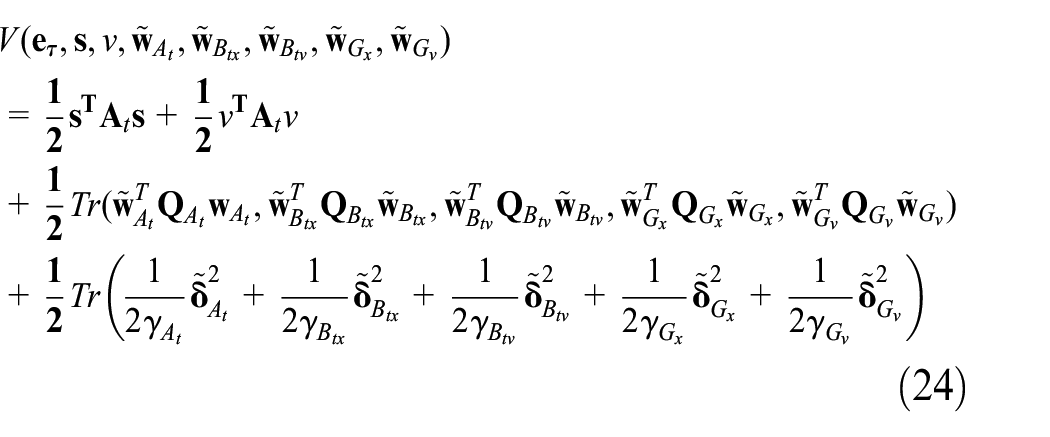
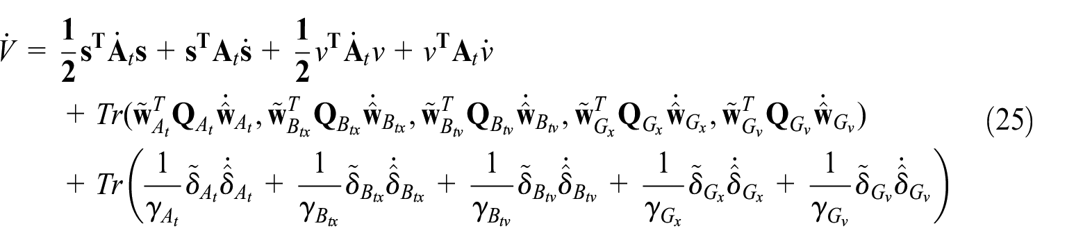
where ${\tilde{\mathbf{w}}}_{(.)}={\hat{\mathbf{w}}}_{(.)}-{\mathbf{w}}_{(·)}^{*}$ denotes the error of weighting vectors and ${\mathbf{\epsilon }}_1=({\mathbf{\epsilon }}_{A_t},{\mathbf{\epsilon }}_{B_{\mathrm{tx}}},{\mathbf{\epsilon }}_{G_x})$ , ${\mathbf{\epsilon }}_2=({\mathbf{\epsilon }}_{B_{\mathrm{tv}}},{\mathbf{\epsilon }}_{G_v})$ denote the lumped approximation errors of A _t , B _tx , B _tv , G _x , and G _v . The Lyapunov candidate function is chosen as

$$\begin{array}{c}V({\mathbf{e}}_{\tau },\mathbf{s},v,{\tilde{\mathbf{w}}}_{A_t},{\tilde{\mathbf{w}}}_{B_{\mathrm{tx}}},{\tilde{\mathbf{w}}}_{B_{\mathrm{tv}}},{\tilde{\mathbf{w}}}_{G_x},{\tilde{\mathbf{w}}}_{G_v})\hfill \\ =\frac{1}{2}{\mathbf{s}}^{\mathbf{T}}{\mathbf{A}}_t\mathbf{s}+\frac{1}{2}{v}^{\mathbf{T}}{\mathbf{A}}_{t}v\hfill \\ +\frac{1}{2}\mathrm{Tr}({\tilde{\mathbf{w}}}_{A_t}^T{\mathbf{Q}}_{A_t}{\mathbf{w}}_{A_t},{\tilde{\mathbf{w}}}_{B_{\mathrm{tx}}}^T{\mathbf{Q}}_{B_{\mathrm{tx}}}{\tilde{\mathbf{w}}}_{B_{\mathrm{tx}}},{\tilde{\mathbf{w}}}_{B_{\mathrm{tv}}}^T{\mathbf{Q}}_{B_{\mathrm{tv}}}{\tilde{\mathbf{w}}}_{B_{\mathrm{tv}}},{\tilde{\mathbf{w}}}_{G_x}^T{\mathbf{Q}}_{G_x}{\tilde{\mathbf{w}}}_{G_x},{\tilde{\mathbf{w}}}_{G_v}^T{\mathbf{Q}}_{G_v}{\tilde{\mathbf{w}}}_{G_v})\hfill \\ +\frac{1}{2}\mathrm{Tr}(\frac{1}{2{\gamma }_{A_t}}{\tilde{\mathbf{\delta }}}_{A_t}^2+\frac{1}{2{\gamma }_{B_{\mathrm{tx}}}}{\tilde{\mathbf{\delta }}}_{B_{\mathrm{tx}}}^2+\frac{1}{2{\gamma }_{B_{\mathrm{tv}}}}{\tilde{\mathbf{\delta }}}_{B_{\mathrm{tv}}}^2+\frac{1}{2{\gamma }_{G_x}}{\tilde{\mathbf{\delta }}}_{G_x}^2+\frac{1}{2{\gamma }_{G_v}}{\tilde{\mathbf{\delta }}}_{G_v}^2)\hfill \end{array}$$

(24)

Tr (.) is the trace operation. Then, the time derivative of (24) along the system trajectory is

$$\begin{array}{cc}\multicolumn{1}{c}{\stackrel{·}{V}=}& \frac{1}{2}{\mathbf{s}}^{\mathbf{T}}{\stackrel{·}{\mathbf{A}}}_t\mathbf{s}+{\mathbf{s}}^{\mathbf{T}}{\mathbf{A}}_t\stackrel{·}{\mathbf{s}}+\frac{1}{2}{v}^{\mathbf{T}}{\stackrel{·}{\mathbf{A}}}_{t}v+v^{\mathbf{T}}{\mathbf{A}}_t\stackrel{·}{v}\hfill \\ \multicolumn{1}{c}{}& +\mathrm{Tr}({\tilde{\mathbf{w}}}_{A_t}^T{\mathbf{Q}}_{A_t}{\stackrel{·}{\hat{\mathbf{w}}}}_{A_t},{\tilde{\mathbf{w}}}_{B_{\mathrm{tx}}}^T{\mathbf{Q}}_{B_{\mathrm{tx}}}{\stackrel{·}{\hat{\mathbf{w}}}}_{B_{\mathrm{tx}}},{\tilde{\mathbf{w}}}_{B_{\mathrm{tv}}}^T{\mathbf{Q}}_{B_{\mathrm{tv}}}{\stackrel{·}{\hat{\mathbf{w}}}}_{B_{\mathrm{tv}}},{\tilde{\mathbf{w}}}_{G_x}^T{\mathbf{Q}}_{G_x}{\stackrel{·}{\hat{\mathbf{w}}}}_{G_x},{\tilde{\mathbf{w}}}_{G_v}^T{\mathbf{Q}}_{G_v}{\stackrel{·}{\hat{\mathbf{w}}}}_{G_v})\hfill \\ \multicolumn{1}{c}{}& +\mathrm{Tr}(\frac{1}{{\gamma }_{A_t}}{\tilde{\delta }}_{A_t}{\stackrel{·}{\hat{}}\delta }_{A_t}+\frac{1}{{\gamma }_{B_{\mathrm{tx}}}}{\tilde{\delta }}_{B_{\mathrm{tx}}}{\stackrel{·}{\hat{}}\delta }_{B_{\mathrm{tx}}}+\frac{1}{{\gamma }_{B_{\mathrm{tv}}}}{\tilde{\delta }}_{B_{\mathrm{tv}}}{\stackrel{·}{\hat{}}\delta }_{B_{\mathrm{tv}}}+\frac{1}{{\gamma }_{G_x}}{\tilde{\delta }}_{G_x}{\stackrel{·}{\hat{}}\delta }_{G_x}+\frac{1}{{\gamma }_{G_v}}{\tilde{\delta }}_{G_v}{\stackrel{·}{\hat{}}\delta }_{G_v})\hfill \end{array}$$

(25)

We use (23) to yield

$$\begin{array}{cc}\multicolumn{1}{c}{\stackrel{·}{V}=}& \frac{1}{2}{\mathbf{s}}^{\mathbf{T}}{\stackrel{·}{\mathbf{A}}}_t\mathbf{s}+\frac{1}{2}{v}^{\mathbf{T}}{\stackrel{·}{\mathbf{A}}}_{t}v\hfill \\ \multicolumn{1}{c}{}& +{\mathbf{s}}^{\mathbf{T}}({\tilde{\mathbf{w}}}_{A_t}{\mathbf{ѱ}}_{A_t}({\stackrel{··}{\mathbf{x}}}_d-\mathbf{k}\stackrel{·}{\mathbf{e}})+{\tilde{\mathbf{w}}}_{B_{\mathrm{tx}}}{\mathbf{ѱ}}_{B_{\mathrm{tx}}}({\stackrel{·}{\mathbf{x}}}_d-\mathbf{ke})-{\mathbf{B}}_{\mathrm{tx}}\mathbf{s}+{\tilde{\mathbf{w}}}_{G_x}{\mathbf{ѱ}}_{G_x}-{\mathbf{B}}_{x}v-{\mathbf{k}}_d\mathbf{s}+{\mathbf{F}}_{x\_\mathrm{robust}}+{\mathbf{\epsilon }}_1)\hfill \\ \multicolumn{1}{c}{}& +v^{\mathbf{T}}({\tilde{\mathbf{w}}}_{B_{\mathrm{tv}}}{\mathbf{ѱ}}_{B_{\mathrm{tv}}}({\stackrel{·}{\mathbf{x}}}_d-\mathbf{ke})-{\mathbf{B}}_{\mathrm{tv}}\mathbf{s}+{\tilde{\mathbf{w}}}_{G_v}{\mathbf{ѱ}}_{G_v}-{\mathbf{B}}_{v}v-{\mathbf{k}}_{n}v+{\mathbf{\delta }}_2+{\mathbf{F}}_{n\_\mathrm{robust}}+{\mathbf{\epsilon }}_2)\hfill \\ \multicolumn{1}{c}{}& +\mathrm{Tr}({\tilde{\mathbf{w}}}_{A_t}^T{\mathbf{Q}}_{A_t}{\stackrel{·}{\hat{\mathbf{w}}}}_{A_t},{\tilde{\mathbf{w}}}_{B_{\mathrm{tx}}}^T{\mathbf{Q}}_{B_{\mathrm{tx}}}{\stackrel{·}{\hat{\mathbf{w}}}}_{B_{\mathrm{tx}}},{\tilde{\mathbf{w}}}_{B_{\mathrm{tv}}}^T{\mathbf{Q}}_{B_{\mathrm{tv}}}{\stackrel{·}{\hat{\mathbf{w}}}}_{B_{\mathrm{tv}}},{\tilde{\mathbf{w}}}_{G_x}^T{\mathbf{Q}}_{G_x}{\stackrel{·}{\hat{\mathbf{w}}}}_{G_x},{\tilde{\mathbf{w}}}_{G_v}^T{\mathbf{Q}}_{G_v}{\stackrel{·}{\hat{\mathbf{w}}}}_{G_v})\hfill \\ \multicolumn{1}{c}{}& +\mathrm{Tr}(\frac{1}{{\gamma }_{A_t}}{\tilde{\delta }}_{A_t}{\stackrel{·}{\hat{}}\delta }_{A_t}+\frac{1}{{\gamma }_{B_{\mathrm{tx}}}}{\tilde{\delta }}_{B_{\mathrm{tx}}}{\stackrel{·}{\hat{}}\delta }_{B_{\mathrm{tx}}}+\frac{1}{{\gamma }_{B_{\mathrm{tv}}}}{\tilde{\delta }}_{B_{\mathrm{tv}}}{\stackrel{·}{\hat{}}\delta }_{B_{\mathrm{tv}}}+\frac{1}{{\gamma }_{G_x}}{\tilde{\delta }}_{G_x}{\stackrel{·}{\hat{}}\delta }_{G_x}+\frac{1}{{\gamma }_{G_v}}{\tilde{\delta }}_{G_v}{\stackrel{·}{\hat{}}\delta }_{G_v})\hfill \end{array}$$

(26)

Since M is positive definite and $\stackrel{·}{\mathbf{M}}-2\mathbf{C}$ is skew-symmetric, the corresponding kinematic equation of the task space and null space should maintain the original property of the physical system. Thus, we have

$$\left[\begin{array}{cc}{\stackrel{·}{\mathbf{A}}}_t\hfill & 0\hfill \\ \multicolumn{1}{c}{0}& {\stackrel{·}{\mathbf{A}}}_v\hfill \end{array}\right]-2\left[\begin{array}{cc}{\mathbf{B}}_{\mathrm{tx}}\hfill & {\mathbf{B}}_{\mathrm{xv}}\hfill \\ \multicolumn{1}{c}{{\mathbf{B}}_{\mathrm{tv}}}& {\mathbf{B}}_v\hfill \end{array}\right]=\left[\begin{array}{cc}{\stackrel{·}{\mathbf{A}}}_t-2{\mathbf{B}}_{\mathrm{tx}}\hfill & -2{\mathbf{B}}_{\mathrm{xv}}\hfill \\ \multicolumn{1}{c}{-2{\mathbf{B}}_{\mathrm{tv}}}& {\stackrel{·}{\mathbf{A}}}_v-2{\mathbf{B}}_v\hfill \end{array}\right]$$

(27)

Note that ${\stackrel{·}{\mathbf{A}}}_t-2{\mathbf{B}}_{\mathrm{tx}}$ and ${\stackrel{·}{\mathbf{A}}}_v-2{\mathbf{B}}_v$ are skew-symmetric matrices and ${\mathbf{B}}_{\mathrm{xv}}=-{\mathbf{B}}_{\mathrm{tv}}^T$ , we have

$$\begin{array}{c}\stackrel{.}{V}={\mathbf{s}}^{\mathbf{T}}\left({\stackrel{.}{\mathbf{A}}}_t-2{\mathbf{B}}_{tx}\right)\mathbf{s}+v^{\mathbf{T}}\left({\stackrel{.}{\mathbf{A}}}_t-2{\mathbf{B}}_v\right)v\\ +{\mathbf{s}}^{\mathbf{T}}\left({\tilde{\mathbf{w}}}_{A_t}{\mathbf{\psi }}_{A_t}\left({\stackrel{··}{\mathbf{x}}}_d-\mathbf{k}\stackrel{.}{e}\right)+{\tilde{\mathbf{w}}}_{B_{tx}}{\mathbf{\psi }}_{B_{tx}}\left({\stackrel{.}{\mathbf{x}}}_d-\mathbf{k}e\right)+{\tilde{\mathbf{w}}}_{G_x}{\mathbf{\psi }}_{G_x}-{\mathbf{B}}_{x}v-{\mathbf{k}}_d\mathbf{s}+{\mathbf{F}}_{x\_robust}+{\mathbf{\epsilon }}_1\right)\\ +v^{\mathbf{T}}\left({\tilde{\mathbf{w}}}_{B_{tv}}{\mathbf{\psi }}_{B_{tv}}\left({\stackrel{.}{\mathbf{x}}}_d-\mathbf{k}e\right)-{\mathbf{B}}_{tv}\mathbf{s}+{\tilde{\mathbf{w}}}_{G_v}{\mathbf{\psi }}_{G_v}-{\mathbf{k}}_{n}v+{\mathbf{F}}_{n\_robust}+{\mathbf{\epsilon }}_2\right)\\ +Tr({\tilde{\mathbf{w}}}_{A_t}^T{\mathbf{Q}}_{A_t}{\stackrel{.}{\widehat{\mathbf{w}}}}_{A_t},{\tilde{\mathbf{w}}}_{B_{tx}}^T{\mathbf{Q}}_{B_{tx}}{\stackrel{.}{\widehat{\mathbf{w}}}}_{B_{tx}},{\tilde{\mathbf{w}}}_{B_{tv}}^T{\mathbf{Q}}_{B_{tv}}{\stackrel{.}{\widehat{\mathbf{w}}}}_{B_{tv}},{\tilde{\mathbf{w}}}_{G_x}^T{\mathbf{Q}}_{G_x}{\stackrel{.}{\widehat{\mathbf{w}}}}_{G_x},{\tilde{\mathbf{w}}}_{G_v}^T{Q}_{G_v}{\stackrel{.}{\widehat{\mathbf{w}}}}_{G_v})\\ +Tr\left(\frac{1}{{\gamma }_{A_t}}{\tilde{\delta }}_{A_t}{\stackrel{.}{\widehat{\delta }}}_{A_t}+\frac{1}{{\gamma }_{B_{tx}}}{\tilde{\delta }}_{B_{tx}}{\stackrel{.}{\widehat{\delta }}}_{B_{tx}}+\frac{1}{{\gamma }_{B_{tv}}}{\tilde{\delta }}_{B_{tv}}{\stackrel{.}{\widehat{\delta }}}_{B_{tv}}+\frac{1}{{\gamma }_{G_x}}{\tilde{\delta }}_{G_x}{\stackrel{.}{\widehat{\delta }}}_{G_x}+\frac{1}{{\gamma }_{G_v}}{\tilde{\delta }}_{G_v}{\stackrel{.}{\widehat{\delta }}}_{G_v}\right)\end{array}$$

(28)

As ${\mathbf{s}}^T{\mathbf{B}}_{\mathrm{xv}}v+v^T{\mathbf{B}}_{\mathrm{tv}}\mathbf{s}=0$ , ${\mathbf{s}}^T({\stackrel{·}{\mathbf{A}}}_t-2{\mathbf{B}}_{\mathrm{tx}})\mathbf{s}=0$ , and $v^T({\stackrel{·}{\mathbf{A}}}_v-2{\mathbf{B}}_v)v=0$ , therefore, (28) is

$$\begin{array}{cc}\multicolumn{1}{c}{\stackrel{·}{V}=}& -{\mathbf{s}}^T{\mathbf{k}}_d\mathbf{s}+{\mathbf{s}}^T({\tilde{\mathbf{w}}}_{A_t}{\mathbf{ѱ}}_{A_t}({\stackrel{··}{\mathbf{x}}}_d-\mathbf{k}\stackrel{·}{\mathbf{e}})+{\tilde{\mathbf{w}}}_{B_{\mathrm{tx}}}{\mathbf{ѱ}}_{B_{\mathrm{tx}}}({\stackrel{·}{\mathbf{x}}}_d-\mathbf{ke})+{\tilde{\mathbf{w}}}_{G_x}{\mathbf{ѱ}}_{G_x}-{\mathbf{B}}_{x}v+{\mathbf{F}}_{x\_\mathrm{robust}}+{\mathbf{\epsilon }}_1)\hfill \\ \multicolumn{1}{c}{}& -v^T{\mathbf{k}}_{n}v+v^T({\tilde{\mathbf{w}}}_{B_{\mathrm{tv}}}{\mathbf{ѱ}}_{B_{\mathrm{tv}}}({\stackrel{·}{\mathbf{x}}}_d-\mathbf{ke})-{\mathbf{B}}_{\mathrm{tv}}\mathbf{s}+{\tilde{\mathbf{w}}}_{G_v}{\mathbf{ѱ}}_{G_v}-{\mathbf{k}}_{n}v+{\mathbf{\delta }}_2+{\mathbf{F}}_{n\_\mathrm{robust}}+{\mathbf{\epsilon }}_2)\hfill \\ \multicolumn{1}{c}{}& +\mathrm{Tr}({\tilde{\mathbf{w}}}_{A_t}^T{\mathbf{Q}}_{A_t}{\stackrel{·}{\hat{\mathbf{w}}}}_{A_t},{\tilde{\mathbf{w}}}_{B_{\mathrm{tx}}}^T{\mathbf{Q}}_{B_{\mathrm{tx}}}{\stackrel{·}{\hat{\mathbf{w}}}}_{B_{\mathrm{tx}}},{\tilde{\mathbf{w}}}_{B_{\mathrm{tv}}}^T{\mathbf{Q}}_{B_{\mathrm{tv}}}{\stackrel{·}{\hat{\mathbf{w}}}}_{B_{\mathrm{tv}}},{\tilde{\mathbf{w}}}_{G_x}^T{\mathbf{Q}}_{G_x}{\stackrel{·}{\hat{\mathbf{w}}}}_{G_x},{\tilde{\mathbf{w}}}_{G_v}^T{\mathbf{Q}}_{G_v}{\stackrel{·}{\hat{\mathbf{w}}}}_{G_v})\hfill \\ \multicolumn{1}{c}{}& +\frac{1}{{\gamma }_{A_t}}{\tilde{\delta }}_{A_t}{\stackrel{·}{\hat{\delta }}}_{A_t}+\frac{1}{{\gamma }_{B_{\mathrm{tx}}}}{\tilde{\delta }}_{B_{\mathrm{tx}}}{\stackrel{·}{\hat{\delta }}}_{B_{\mathrm{tx}}}+\frac{1}{{\gamma }_{B_{\mathrm{tv}}}}{\tilde{\delta }}_{B_{\mathrm{tv}}}{\stackrel{·}{\hat{\delta }}}_{B_{\mathrm{tv}}}+\frac{1}{{\gamma }_{G_x}}{\tilde{\delta }}_{G_x}{\stackrel{·}{\hat{\delta }}}_{G_x}+\frac{1}{{\gamma }_{G_v}}{\tilde{\delta }}_{G_v}{\stackrel{·}{\hat{\delta }}}_{G_v}\hfill \end{array}$$

(29)

If the update laws are chosen from equation (19), we have

$$\begin{array}{cc}\multicolumn{1}{c}{\stackrel{·}{V}=}& -{\mathbf{s}}^T{\mathbf{k}}_d\mathbf{s}-v^T{\mathbf{k}}_{n}v\hfill \\ \multicolumn{1}{c}{}& +{\mathbf{s}}^T({\tilde{\mathbf{w}}}_{A_t}{\mathbf{ѱ}}_{A_t}({\stackrel{··}{\mathbf{x}}}_d-\mathbf{k}\stackrel{·}{\mathbf{e}})+{\tilde{\mathbf{w}}}_{B_{\mathrm{tx}}}{\mathbf{ѱ}}_{B_{\mathrm{tx}}}({\stackrel{·}{\mathbf{x}}}_d-\mathbf{ke})+{\tilde{\mathbf{w}}}_{G_x}{\mathbf{ѱ}}_{G_x}-{\mathbf{B}}_{x}v+{\mathbf{\epsilon }}_1)\hfill \\ \multicolumn{1}{c}{}& +v^T({\tilde{\mathbf{w}}}_{B_{\mathrm{tv}}}{\mathbf{ѱ}}_{B_{\mathrm{tv}}}({\stackrel{·}{\mathbf{x}}}_d-\mathbf{ke})-{\mathbf{B}}_{\mathrm{tv}}\mathbf{s}+{\tilde{\mathbf{w}}}_{G_v}{\mathbf{ѱ}}_{G_v}-{\mathbf{k}}_{n}v+{\mathbf{\epsilon }}_2)\hfill \\ \multicolumn{1}{c}{}& -{\mathbf{s}}^T{\tilde{\mathbf{w}}}_{A_t}^T{\mathbf{ѱ}}_{A_t}({\stackrel{··}{\mathbf{x}}}_d-\mathbf{k}\stackrel{·}{\mathbf{e}})-{\mathbf{s}}^T{\tilde{\mathbf{w}}}_{B_{\mathrm{tx}}}^T{\mathbf{ѱ}}_{B_{\mathrm{tx}}}({\stackrel{·}{\mathbf{x}}}_d-\mathbf{ke})-{\mathbf{s}}^T{\tilde{\mathbf{w}}}_{G_x}^T{\mathbf{ѱ}}_{G_x}\hfill \\ \multicolumn{1}{c}{}& -v^T{\tilde{\mathbf{w}}}_{B_{\mathrm{tv}}}^T{\mathbf{ѱ}}_{B_{\mathrm{tv}}}({\stackrel{·}{\mathbf{x}}}_d-\mathbf{ke})-v^T{\tilde{\mathbf{w}}}_{G_v}^T{\mathbf{ѱ}}_{G_v}\hfill \\ \multicolumn{1}{c}{}& +{\mathbf{s}}^T{\mathbf{F}}_{x\_\mathrm{robust}}+v^T{\mathbf{F}}_{n\_\mathrm{robust}}+\frac{1}{{\gamma }_{A_t}}{\tilde{\delta }}_{A_t}{\stackrel{·}{\hat{\delta }}}_{A_t}+\frac{1}{{\gamma }_{B_{\mathrm{tx}}}}{\tilde{\delta }}_{B_{\mathrm{tx}}}{\stackrel{·}{\hat{\delta }}}_{B_{\mathrm{tx}}}+\frac{1}{{\gamma }_{B_{\mathrm{tv}}}}{\tilde{\delta }}_{B_{\mathrm{tv}}}{\stackrel{·}{\hat{\delta }}}_{B_{\mathrm{tv}}}+\frac{1}{{\gamma }_{G_x}}{\tilde{\delta }}_{G_x}{\stackrel{·}{\hat{\delta }}}_{G_x}+\frac{1}{{\gamma }_{G_v}}{\tilde{\delta }}_{G_v}{\stackrel{·}{\hat{\delta }}}_{G_v}\hfill \end{array}$$

(30)

Note that ${\mathbf{B}}_{\mathrm{xv}}=-{\mathbf{B}}_{\mathrm{tv}}^T$ ; so, we have

$$\begin{array}{cc}\multicolumn{1}{c}{\stackrel{·}{V}=}& -{\mathbf{s}}^T{\mathbf{k}}_d\mathbf{s}-v^T{\mathbf{k}}_{n}v+{\mathbf{s}}^T{\mathbf{\epsilon }}_1+v^T{\mathbf{\epsilon }}_2+{\mathbf{s}}^T{\mathbf{F}}_{x\_\mathrm{robust}}+v^T{\mathbf{F}}_{n\_\mathrm{robust}}\hfill \\ \multicolumn{1}{c}{}& +\frac{1}{{\gamma }_{A_t}}{\tilde{\delta }}_{A_t}{\stackrel{·}{\hat{\delta }}}_{A_t}+\frac{1}{{\gamma }_{B_{\mathrm{tx}}}}{\tilde{\delta }}_{B_{\mathrm{tx}}}{\stackrel{·}{\hat{\delta }}}_{B_{\mathrm{tx}}}+\frac{1}{{\gamma }_{B_{\mathrm{tv}}}}{\tilde{\delta }}_{B_{\mathrm{tv}}}{\stackrel{·}{\hat{\delta }}}_{B_{\mathrm{tv}}}+\frac{1}{{\gamma }_{G_x}}{\tilde{\delta }}_{G_x}{\stackrel{·}{\hat{\delta }}}_{G_x}+\frac{1}{{\gamma }_{G_v}}{\tilde{\delta }}_{G_v}{\stackrel{·}{\hat{\delta }}}_{G_v}\hfill \\ \multicolumn{1}{c}{}& \le -{\mathbf{s}}^T{\mathbf{k}}_d\mathbf{s}-v^T{\mathbf{k}}_{n}v\le 0\hfill \end{array}$$

(31)

As mentioned above, by choosing the positive definite matrix k _d and k _n , the stability of the closed-loop system is guaranteed by the Lyapunov stability theorem, i.e. the tracking error converges to zero such that the state x will follow the desired trajectory x _d .

Adaptive force control via position control

In our analysis, the contact environment is assumed to be unknown, that is, the stiffness coefficient is unknown. Therefore, the adaptive force tracking control is achieved by estimation of stiffness coefficient and position control. According to the results obtained by previous works,^2,6,7 we know that the inertia and damping parameters only have influence on the transient response of target impedance equation; therefore, we can obtain the steady-state response relationship

$${\mathbf{F}}_{\mathrm{ext}}\cong {\mathbf{K}}_e(\mathbf{x}-{\mathbf{x}}_e)$$

(32)

where K _e is the stiffness coefficient of contact environment and x _e is the position of the environment. For the desired force, the relation between the environment and the end-effector position is

$${\mathbf{F}}_d\cong {\mathbf{K}}_e({\mathbf{x}}^{*}-{\mathbf{x}}_e)$$

(33)

where ^x* is the ideal trajectory for the desired force. Thus, we can achieve the force control goal F _ext  = F _d . However, the stiffness coefficient, K _e , of the environment is not exactly known. Hence, we should estimate the stiffness coefficient ${\hat{\mathbf{K}}}_e$ to achieve the force control goal. In this study, we have proposed the adaptive force control to estimate the stiffness coefficient, ${\hat{\mathbf{K}}}_e$ , by gradient descent method, as shown in Figure 1. We first define the force tracking error as

$${\mathbf{e}}_{F_{\mathrm{ext}}}={\mathbf{F}}_d-{\mathbf{F}}_{\mathrm{ext}}$$

(34)

and simplify the force in one direction for a clearer description. Thus, ${\hat{K}}_e$ is the scalar element of ${\hat{\mathbf{K}}}_e$ and $e_{F_{\mathrm{ext}}}=f_d-f_{\mathrm{ext}}$ . The Lyapunov candidate function of force control is

$$V_{F_{\mathrm{ext}}}=\frac{1}{2}{\mathbf{e}}_{F_{\mathrm{ext}}}^T{\mathbf{e}}_{F_{\mathrm{ext}}}$$

(35)

and

$$\frac{\partial V_{F_{\mathrm{ext}}}}{\partial {\hat{K}}_e}=\frac{\partial e_{F_{\mathrm{ext}}}}{\partial {\hat{K}}_e}\times e_{F_{\mathrm{ext}}}$$

(36)

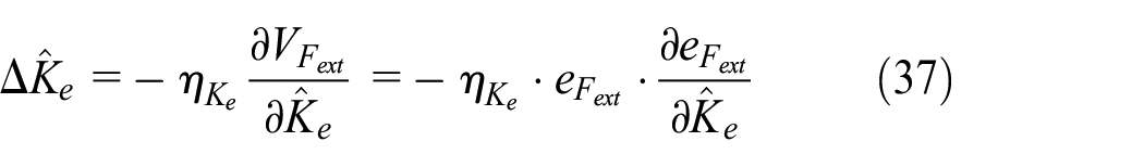
By the gradient descent method, the update of stiffness coefficient ${\hat{\mathbf{K}}}_e$ is

$$\mathrm{\Delta }{\hat{K}}_e=-{\eta }_{K_e}\frac{\partial V_{F_{\mathrm{ext}}}}{\partial {\hat{K}}_e}=-{\eta }_{K_e}·e_{F_{\mathrm{ext}}}·\frac{\partial e_{F_{\mathrm{ext}}}}{\partial {\hat{K}}_e}$$

(37)

where ${\eta }_{K_e}$ denotes the update parameter. The update parameter concerns the convergence reaction, which means the smaller value of ${\eta }_{K_e}$ causes slower convergence and the bigger one causes the unstable result.

Thus, we have the following theorem for adaptive force tracking control.

Theorem 2

Considering the redundant robot manipulator, the adaptive force control is guaranteed if the update parameter ${\eta }_{K_e}$ satisfies

$$0<\frac{{\eta }_{K_e}}{2}{\left(\frac{\partial e_{F_{\mathrm{ext}}}}{\partial {\hat{K}}_e}\right)}^2<1$$

(38)

Proof

As discussed above, one-dimensional external force is considered, and we have the Lyapunov candidate

$$V_{F_{\mathrm{ext}}}\left(k\right)=\frac{1}{2}{(f_d\left(k\right)-f_{\mathrm{ext}}\left(k\right))}^2$$

(39)

where k is the time-instant for parameters update. Let $\mathrm{\Delta }{e}_{F_{\mathrm{ext}}}\left(k\right)=e_{F_{\mathrm{ext}}}(k+1)-e_{F_{\mathrm{ext}}}\left(k\right)$ , we obtain

$$\begin{array}{cc}\multicolumn{1}{c}{\mathrm{\Delta }{V}_{F_{\mathrm{ext}}}\left(k\right)}& =V_{F_{\mathrm{ext}}}(k+1)-V_{F_{\mathrm{ext}}}\left(k\right)\hfill \\ \multicolumn{1}{c}{}& =\frac{1}{2}{(f_d(k+1)-f_{\mathrm{ext}}(k+1))}^2-\frac{1}{2}{(f_d\left(k\right)-f_{\mathrm{ext}}\left(k\right))}^2\hfill \\ \multicolumn{1}{c}{}& =\frac{1}{2}[{\left(e_{F_{\mathrm{ext}}}(k+1)\right)}^2-{\left(e_{F_{\mathrm{ext}}}\left(k\right)\right)}^2]\hfill \\ \multicolumn{1}{c}{}& =\frac{1}{2}[e_{F_{\mathrm{ext}}}(k+1)+e_{F_{\mathrm{ext}}}\left(k\right)][e_{F_{\mathrm{ext}}}(k+1)-e_{F_{\mathrm{ext}}}\left(k\right)]\hfill \\ \multicolumn{1}{c}{}& =\frac{1}{2}[2e_{F_{\mathrm{ext}}}\left(k\right)+\mathrm{\Delta }{e}_{F_{\mathrm{ext}}}\left(k\right)]·\mathrm{\Delta }{e}_{F_{\mathrm{ext}}}\left(k\right)\hfill \\ \multicolumn{1}{c}{}& =\frac{1}{2}\mathrm{\Delta }{e}_{F_{\mathrm{ext}}}^2\left(k\right)+e_{F_{\mathrm{ext}}}\left(k\right)·\mathrm{\Delta }{e}_{F_{\mathrm{ext}}}\left(k\right)\hfill \end{array}$$

(40)

According to the gradient descent method, we have, $\mathrm{\Delta }{e}_{F_{\mathrm{ext}}}\left(k\right)\approx \frac{\partial e_{F_{\mathrm{ext}}}}{\partial {\hat{K}}_e}\mathrm{\Delta }{\hat{K}}_e$ and $\mathrm{\Delta }{\hat{K}}_e=-{\eta }_{K_e}\frac{\partial V_{F_{\mathrm{ext}}}}{\partial {\hat{K}}_e}=-{\eta }_{K_e}{e}_{F_{\mathrm{ext}}}\left(\frac{\partial e_{F_{\mathrm{ext}}}}{\partial {\hat{K}}_e}\right)$ ; thus

$$\mathrm{\Delta }{V}_{F_{\mathrm{ext}}}\left(k\right)=-{\eta }_{K_e}{e}_{F_{\mathrm{ext}}}^2{\left(\frac{\partial e_{F_{\mathrm{ext}}}}{\partial {\hat{K}}_e}\right)}^2(1-\frac{1}{2}{\eta }_{K_e}{\left(\frac{\partial e_{F_{\mathrm{ext}}}}{\partial {\hat{K}}_e}\right)}^2)$$

(41)

We can guarantee the stability if the update parameter of stiffness coefficient satisfies equation (38) such that $\mathrm{\Delta }{V}_{F_{\mathrm{ext}}}\left(k\right)\le 0$ , $\forall k>0$ . This means that the force error (34) will converge to zero when k approaches infinity.

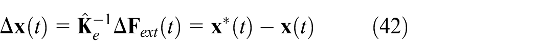
Our purpose is to find the desired trajectory ${\mathbf{x}}_d^{*}$ , that is, F _ext  = F_d. In order to achieve the force control in the contact space, we can obtain $\mathrm{\Delta }\mathbf{x}$ , which is between reference trajectory and real trajectory, as

$$\mathrm{\Delta }\mathbf{x}\left(t\right)={\hat{\mathbf{K}}}_e^{-1}\mathrm{\Delta }{\mathbf{F}}_{\mathrm{ext}}\left(t\right)={\mathbf{x}}^{*}\left(t\right)-\mathbf{x}\left(t\right)$$

(42)

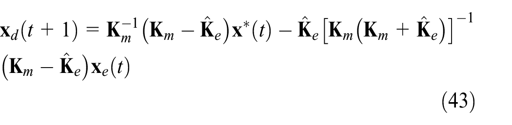
where the force error $\mathrm{\Delta }{\mathbf{F}}_{\mathrm{ext}}={\mathbf{F}}_d-{\mathbf{F}}_{\mathrm{ext}}$ . We design the reference trajectory to accomplish force control ${\mathbf{x}}^{*}\left(t\right)=\mathbf{x}\left(t\right)+\mathrm{\Delta }\mathbf{x}\left(t\right)$ . According to the target impedance equation, we obtain the new desired trajectory as

$$\begin{array}{c}{\mathbf{x}}_d(t+1)={\mathbf{K}}_m^{-1}({\mathbf{K}}_m-{\hat{\mathbf{K}}}_e){\mathbf{x}}^{*}\left(t\right)-{\hat{\mathbf{K}}}_e{\left[{\mathbf{K}}_m({\mathbf{K}}_m+{\hat{\mathbf{K}}}_e)\right]}^{-1}\hfill \\ ({\mathbf{K}}_m-{\hat{\mathbf{K}}}_e){\mathbf{x}}_e\left(t\right)\hfill \end{array}$$

(43)

Therefore, we can achieve the adaptive force control by an update of the stiffness coefficient ${\hat{\mathbf{K}}}_e$ and desired trajectory. Above all, the end-effector of redundant robot manipulator will track the desired trajectory.

Simulation results

This section introduces the simulation results of a redundant robot manipulator, KUKA lightweight robot (LWR).^22,23 The KUKA LWR has a 7-link robot manipulator, that is, n = 7 and r = 1 (redundancy), and the Lagrangian dynamic formulation and system parameters are used here.^1,22,23 To illustrate the performance of our approach, we have applied the proposed adaptive force control scheme on the redundant KUKA LWR.

The initial desired conditions are q _d (0) = [10 20 30 10 50 60 70] × π/180 and x _d (0) = [−0.0498 0.0688 0.7916 2.5670 −2.7584 −0.392]. We consider the tracking control problem with initial condition errors as q (0) = [10 20 30 10 50 60 70] × π/180, x (0) = [−0.0474 0.0801 0.7988 2.8033 −2.7479 −0.5963]. The initial weighting vector of fuzzy systems are randomly chosen in [0 1]. The fuzzy rule numbers are all chosen as 9. The update laws gain matrices are

$$\begin{array}{c}{\mathbf{Q}}_{A_t}^{-1}=\mathrm{diag}(q_1,\dots ,q_i),q_i={10}^{-6},i=1,\dots ,9\hfill \\ {\mathbf{Q}}_{B_{\mathrm{tx}}}^{-1}=\mathrm{diag}(q_1,\dots ,q_i),q_i={10}^{-6},i=1,\dots ,9\hfill \\ {\mathbf{Q}}_{B_{\mathrm{tv}}}^{-1}=\mathrm{diag}(q_1,\dots ,q_i),q_i={10}^{-3},i=1,\dots ,9\hfill \\ {\mathbf{Q}}_{G_x}^{-1}=\mathrm{diag}(q_1,\dots ,q_i),q_i={10}^{-6},i=1,\dots ,9\hfill \\ {\mathbf{Q}}_{G_v}^{-1}=\mathrm{diag}(q_1,\dots ,q_i),q_i={10}^{-3},i=1,\dots ,9\hfill \end{array}$$

The desired force F _d is selected as 5 N. The control gain matrices and environment stiffnesses are selected as k = diag (25, 25, 45, 30, 140, 40) and k _d  = diag (80, 80, 80, 10⁻⁵, 10⁻⁴, 10⁻⁴), respectively. The matrices of the target impedance are selected as k _n  = 25, K _e  = 300 N/m, and K _m  = 1.5 × 10⁵. As above, we assume that the dynamic model matrices A _t , B _tx , B _tv , G _x , and G _v are not exactly known and are estimated using established fuzzy systems denoting them ${\hat{\mathbf{A}}}_t$ , ${\hat{\mathbf{B}}}_{\mathrm{tx}}$ , ${\hat{\mathbf{B}}}_{\mathrm{tv}}$ , ${\hat{\mathbf{G}}}_x$ , and ${\hat{\mathbf{G}}}_v$ . Note that ${\hat{\mathbf{A}}}_t$ , ${\hat{\mathbf{B}}}_{\mathrm{tx}}$ , ${\hat{\mathbf{B}}}_{\mathrm{tv}}$ , ${\hat{\mathbf{G}}}_x$ , and ${\hat{\mathbf{G}}}_v$ are all matrix forms, each element is estimated by a fuzzy system by adaptive scheme.

To show the effectiveness of our approach by simulation results, we used MATLAB software (KUKA LWR4) as shown in Figure 2. Figure 3 shows the simulation results of tracking control with initial error. Figure 3(a) shows the trajectory of the end-effector (blue solid line: reference; red solid line: actual response). It can be seen that a small tracking error occurs on the Z-axis due to the force tracking (F _d  = 5 N). It can also be found on the corresponding trajectories and tracking errors as shown in Figure 3(b). From Figure 3(a) and (b), we can see that the performance and effectiveness of our control scheme is robust. The initial errors converge rapidly in 1 s and the end-effector contacts the environment in the third second. The corresponding joint torque of the robot manipulator is introduced in Figure 3(c), since the trajectory is planned by cubic spline to lead the position, velocity and acceleration continuous and also contact the environment in the third second. In addition, from Figure 3(c), we can see that the velocity of the second joint is maintained at zero to make the second joint constant. Moreover, we find that the end-effector contacts the environment in the third second and the force can track to the desired force. Figure 3(d) is the contact force of end-effector and shows the performance of the proposed adaptive force control. After the end-effector contacts the environment, the force tracking is achieved in 0.5 s. The corresponding estimated stiffness coefficient ${\hat{\mathbf{K}}}_e$ is shown in Figure 3(e). From the results of Figure 3(e), we can observe that the force tracking approach results in good performance and the estimated stiffness converges to the desired one.

Figure 2.

The simulation of robot manipulator using MATLAB.

Figure 3.

Simulation results of force tracking control with initial error: (a) trajectory tracking performance in the task space, (b) tracking error, (c) joint trajectories, (d) force tracking results, and (e) stiffness coefficient tracking performance.

As discussed above, adaptive force control can be achieved by our adaptive algorithm and the estimation of the ideal trajectory for the desired force, ${\mathbf{x}}^{*}$ , through the estimation of stiffness. We now introduce the discussion of update parameters (Figure 4). As shown in Figure 4(a), we have the different update parameters for the estimated stiffness coefficient ${\hat{\mathbf{K}}}_e$ and the results of force tracking control (Case 1: ${\eta }_{k_e}=0.0003$ , Case 2: ${\eta }_{k_e}=0.003$ , Case 3: ${\eta }_{k_e}=0.03$ , and Case 4: ${\eta }_{k_e}=0.08$ ). It can be seen from Figure 4(a) and (b) that a small value of ${\eta }_{k_e}$ causes slower convergence and the force control behavior has a longer raising time, while a large value causes quick convergence and the overshooting of force, which can damage the workpiece or machine. Thus, choosing a suitable value of the update parameter ${\eta }_{k_e}$ is important. From the results obtained in Figure 4(a) and (b), we suggest the update parameter ${\eta }_{k_e}=0.03$ , which performs well in the estimation of stiffness coefficient as the force control behavior has small raising time and overshoot. Figure 4(c) shows the velocity of the joint. Considering the constraint, ²² the velocity of the joint is not out of range. Figure 4(d) shows the results of the null space velocity.

Figure 4.

Discussion of update parameters for force tracking: (a) estimation of ${\hat{K}}_e$ , (b) force tracking trajectories, (c) velocities of joints, and (d) velocity of the null space.

Conclusion

This article has proposed an adaptive force controller design for a redundant robot manipulator operating in an uncertain and unknown task space. The relation between the task and joint spaces was introduced to derive the dynamic model of task and null space. We have utilized the position and force controller design to overcome these problems by adaptive fuzzy systems. For adaptive force control, the stiffness coefficient of the environment is unknown; therefore, the gradient descent method is used to estimate the stiffness coefficient of environment to achieve the adaptive force tracking control. The stability analysis of the closed-loop system and the corresponding update laws are given by Lyapunov stability theorem. Finally, several simulations using the KUKA LWR4 were performed to validate our approach and demonstrate the performance and effectiveness of our proposed system.