Sage Journals: Discover world-class research

Abstract

Many structures are subjected to the risk of fatigue failure. For their reliability-based design, it is thus important to calculate the probability of fatigue failure and assess the relative importance of the involved parameters. Although various studies have analyzed the fatigue failure, the stage of fracture failure has been less focused. In particular, the risk analysis of fracture failure needs to be conducted considering its importance in actual structures. This article proposes a new probabilistic framework for the risk and sensitivity analysis of structural fatigue failure employing cohesive zone elements. The proposed framework comprises three steps, namely finite element analysis using cohesive zone elements, response surface construction, and risk and sensitivity analysis of fatigue failure, which require several mathematical techniques and algorithms. The proposed framework is tested by applying it to an illustrative example, and the corresponding analysis results of fracture failure probability with different threshold values of a limit-state function are presented. In addition, the sensitivities of failure risk with respect to the statistical parameters of random variables are presented and their relative importance is discussed.

Keywords

Fracture failure cohesive zone element finite element analysis response surface risk and sensitivity

Introduction

Fatigue is one of the main causes of structural failure. Many structures in various engineering disciplines are subjected to the risk of fatigue-induced failure caused by repeated loading over their life cycle.¹ When a structure is subjected to repeated loading over its lifetime, a local crack may propagate and lead to a disproportionally large damage such as structural collapse. Therefore, an adequate level of structural safety should be provided to prevent such a fatigue-induced structural failure from causing significant loss.

One of the most widely used approaches for fatigue analysis is based on the S-N curve, which has been presented in several studies.^2,3 This method is also called the “stress-life” method and has been developed as a “safe-life” approach for the design against fatigue.⁴ Although the S-N curve has been applied to various structures and has been proven to be effective since its development, the fatigue life of structures cannot be determined with sufficient accuracy because various sources of uncertainties (i.e. random variables (RVs)) are involved in the fatigue process. During an S-N test, it is observed that the same material specimen fails after different numbers of cycles over the same range of applied stress, and a large amount of these uncertainties are mainly due to material inhomogeneity.⁵ Hence, the application of statistical and probabilistic theories is challenging to account for these uncertainties. Because of the scatter in the S-N experimental data, the mean of the probabilistic distribution of the number of cycles, N, is plotted against the stress range, S, to obtain a meaningful S-N curve. Because S-N curve experiments are relatively easy and inexpensive to conduct, a vast amount of experimental S-N data exists for most materials.

Another important approach that has been widely used for fatigue analysis is the Paris equation, which accounts for the crack propagation rate and is based on the fracture mechanics theory.⁶ The introduction of the Paris equation was an important breakthrough because it facilitates the characterization of fatigue crack growth and allows for the assessment of service life or inspection intervals required under definite loading conditions and service environments. Hence, the Paris equation has been applied to various steel structures including bridges,⁷ aircraft,⁸ ship structures,⁹ offshore platforms,^10,11 and wind turbine blades.¹²

In this approach, the fatigue failure process is classified into three stages: (1) crack initiation stage (i.e. Stage I), which involves crack nucleation and short crack propagation; (2) crack propagation stage (i.e. Stage II), which involves propagation of long cracks; and (3) fracture stage (i.e. Stage III), in which the failure occurs due to an extremely high crack propagation rate. Although the Paris equation has been applied to various structural problems, it cannot be applied to the crack initiation and fracture stages. To overcome this limitation, advanced models have been proposed by several researchers including Dowling et al.,¹³ Klesnil and Lukáš,¹⁴ and Donahue et al.¹⁵ However, there is still a limitation on the analysis of the fracture stage (i.e. Stage III), because the increase in the crack propagation rate is considerable. As such, considering that this is the stage in which a structure actually fails, it is very important to introduce a sophisticated method to deal with the fracture stage in the fatigue analysis.

For this reason, cohesive zone modeling (CZM) was developed and has been widely used.^16,17 Although CZM is a powerful method to analyze fatigue and fracture, many uncertainties are involved.^18,19 The uncertainties related to fatigue become more evident from the scatter in the S-N data, and a statistical and probabilistic approach is required to account for these uncertainties.

This article proposes a new probabilistic framework for the risk and sensitivity analysis of fracture failure employing cohesive zone elements (CZEs). As listed in Table 1, the proposed framework comprises three steps: (1) finite element analysis; (2) response surface construction; and (3) risk and sensitivity quantification, which require several numerical methods and computational tools.

Table 1.

Overview of the proposed framework for probabilistic fracture analysis.

Step	Task	Method	Computational tool
1	Finite element analysis	Cohesive zone element	ABAQUS^®
2	Response surface construction	Response surface method	MATLAB–ABAQUS
3	Risk and sensitivity quantification	First-order reliability method	FERUM

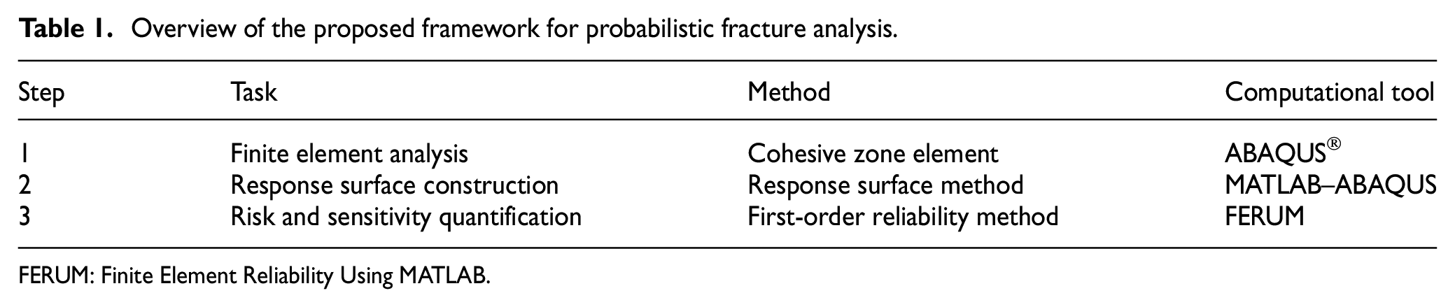
FERUM: Finite Element Reliability Using MATLAB.

In the first step, that is, finite element analysis, a model, which can appropriately represent the fatigue and fracture behaviors of a structure, is built. For this task, a finite element model for ABAQUS^® is constructed using CZEs, and the details can be found in section “Finite element analysis employing CZEs.” The second step, that is, response surface construction, focuses on deriving an analytical function (the so-called response surface function), which can approximate the relationship between the uncertainty sources (i.e. RVs) and the structural quantity of the interests. This method is often called the response surface method (RSM), and it requires performing repeated finite element analyses with different values of RVs. For this task, a new computational platform, termed the MATLAB-ABAQUS, is developed by connecting MATLAB^® and ABAQUS, the details of which are described in section “Response surface construction.” In the third step, that is, risk and sensitivity analysis, the failure probability of a structure and its sensitivity with respect to the statistical parameters (e.g. mean and standard deviation) of each RV are determined, and first-order reliability method (FORM), which is one of the widely used reliability analysis methods, is introduced with a reliability analysis software package, namely Finite Element Reliability Using MATLAB (FERUM). The details of this are given later in this article.

Proposed framework

Finite element analysis employing CZEs

As mentioned previously, one of the most widely used models to analyze fatigue crack propagation is the Paris equation, which provides a phenomenological relationship between the crack growth rate and the stress intensity factor range. Several numerical methods have been developed to calculate the stress intensity factor for a complex structure by incorporating one or several cracks, for example, the finite element alternating method²⁰ and the extended finite element method.²¹ Such methods can be used in combination with the Paris equation to model fatigue crack growth.^22,23 However, the use of the Paris equation is limited because the equation is applicable only when specific requirements are met; a long initial crack must be present and the yielding at the crack tip must be limited. In reality, however, initial cracks can exist in a structure for several reasons, including manufacturing defects, voids in welds, and metallurgical discontinuities.³ Furthermore, the initial crack length is known to possess uncertainty and is often considered as an RV.^8,11

A cohesive element, which was developed by Dugdale¹⁶ and Barenblatt,¹⁷ is an alternative method to account for the crack growth and fracture via finite element simulation. In the method, cohesive elements are assumed to be zero-thickness elements inserted between the bulk elements and account for the resistance to crack opening by following a dedicated traction displacement law. The cohesive force dissipates, at least partially, the energy associated with crack formation. De Borst et al.²⁴ introduced a partition of a unity-based approach, which allows modeling the cohesive cracks independently from the mesh.

However, the cohesive elements described above are unsuitable for modeling fatigue crack growth. In such cases, the parameters of the finite element model no longer vary after a few cycles, leading to crack arrest. Nguyen et al.²⁵ extended the cohesive law to include fatigue crack growth. To account for fatigue crack growth, the material properties at each cycle were assumed to deteriorate. During the unloading–reloading process, a hysteresis loop is induced as per the cohesive law, and a slight reduction in the stiffness results in fatigue crack propagation. Such cohesive elements account for both crack initiation and crack propagation.

Hillerborg et al.²⁶ introduced new cohesive elements into a finite element model to simulate a fictitious crack. This model, which has also been referred to as the cohesive zone model, is merely an application of the strip-yield model proposed by Dugdale¹⁶ and Barenblatt.¹⁷ In the Hillerborg model, the stress displacement behavior observed in the damage zone of a tensile specimen is expressed in terms of material property.

At the traction-free crack tip, the damage zone reaches a critical displacement δ_c. The tractions are zero at this point; however, they are equal to the tensile strength at the tip of the damage zone. Assuming that the closure stress σ and opening displacement δ are uniquely related, the energy release rate G for crack growth can be expressed as follows

G = \int_{0}^{δ_{c}} σ d δ

(1)

Whenever the stress or energy release rate of each cohesive element reaches a critical value, the element eventually ruptures and loses its stiffness, and it can be eliminated from the finite element model. Finally, this sequential elimination of the cohesive elements represents crack propagation.

In this study, a finite element model using CZEs is constructed for ABAQUS, which is a commercial software package for finite element analysis. It offers a library of cohesive elements, which can be applied to model various structural behaviors including crack propagation, adhesive joints, and interfaces in composites.²⁷ Among the available elements, in this research, the traction-separation-based modeling of the available features is employed. The cohesive elements help model the initial loading, the initiation of damage, and the propagation of damage, which eventually leads to failure at the bonded interface. The interface behavior prior to the initiation of damage is often described as linear elastic in terms of the penalty stiffness, which decreases under tensile and/or shear loading but is unaffected under pure compression.²⁷

ABAQUS provides the cohesive elements for both two-dimensional (2D) and three-dimensional (3D) modeling, namely COH2D4 and COH3D8, respectively. For 3D problems, three components of separation are assumed in the traction-separation-based model: one normal to the interface and two parallel to it; and the corresponding stress components are assumed to be active at a material point. For 2D problems, two components of separation are assumed in the traction-separation-based model assumes: one normal to the interface and the other parallel to it, and the corresponding stress components are assumed to be active at a material point.²⁷

Response surface construction

The RSM is a set of mathematical and statistical techniques designed to gain a better understanding of the overall response by designing experiments and subsequent analysis of experimental data.^28,29 It uses empirical (non-mechanistic) models, in which the response function is replaced by a simple function (often polynomial), which is fitted to the data for a set of carefully selected points. The RSM is particularly useful for the modeling and analysis of problems in which a response of interest is influenced by several variables and the objective is to optimize the response.

The response surface construction requires performing finite element analysis repeatedly, with different values of the RVs. In this study, as a computational tool, ABAQUS is connected to MATLAB, which is a widely used programming platform. The computational platform is termed MATLAB–ABAQUS. Figure 1 shows the data flow in the platform. First, MATLAB is used to determine the RV values based on their statistical parameters such as mean and standard deviation. Next, ABAQUS input files with the determined RV values are automatically generated and then sent to ABAQUS. Finite element analyses are performed using the input files, and the output responses, for example, force or displacement, evaluated by the structural analysis performed using ABAQUS are obtained. By coupling the two software packages, the proposed framework allows for a more convenient and efficient response surface construction.

Figure 1.

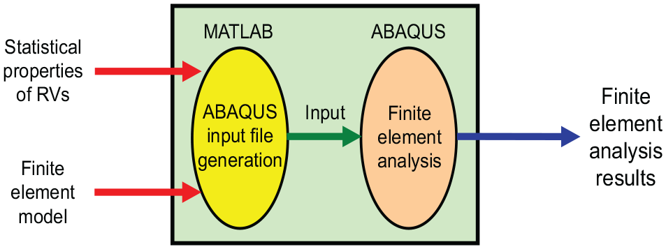
Data flow in MATLAB-ABAQUS.

The RSM can be employed before, during, or after the regression analysis is performed on the data. In the design of experiments (DOEs), it is used before the regression analysis, whereas in the application of optimization techniques, it is used after.

In this study, two types of response surfaces are considered. The first one is a function proposed by Bucher and Bourgund²⁸ and the other one is the central composite design (CCD) function.²⁹ The general formulations are given as

f_{approx} (\cdot) = b_{0} + \sum_{i = 1}^{n} b_{i} x_{i} + \sum_{i = 1}^{n} b_{i} x_{i}^{2}

(2a)

f_{approx} (\cdot) = b_{0} + \sum_{i = 1}^{n} b_{i} x_{i} + \sum_{i = 1}^{n} b_{i} x_{i}^{2} + \sum_{i = 1}^{n - 1} \sum_{j = i + 1}^{n} b_{ij} x_{i} x_{j}

(2b)

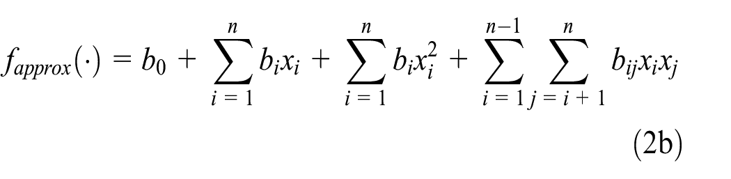
where b₀, b_i, b_ii, and b_ij are coefficients, and x_i and x_j are the values of the RVs. As shown in equations (2a) and (2b), the only difference between the two types of response functions is the additional coupling terms in the CCD function. This makes it possible for the CCD model to represent the true response function more accurately. However, it is also obvious that a greater number of experiments are required to construct the CCD model. For both the response functions, the coefficients can be obtained using equation (3)

{b} = {({[X]}^{T} [X])}^{- 1} {[X]}^{T} {y}

(3)

where b and y are the vectors of the coefficients and simulations, respectively, and X is a matrix constructed from the terms of equation (3) and variables x_i and x_j.

Risk and sensitivity quantification

Once the response surface is constructed, it can be applied to the risk and sensitivity analyses using a reliability analysis method. Different reliability analysis methods have been developed and employed in various engineering disciplines,³⁰ and they can be classified into two groups, namely sampling-based methods and analytical (or non-sampling-based) methods, which can be represented using Monte Carlo simulation (MCS) and FORM, respectively. Melchers³¹ and Der Kiureghian³² have provided detailed reviews on the above two methods. In this article, FORM is introduced to overcome the disadvantages of MCS for the derivation of seismic fragility curves. The methods are briefly introduced in this section.

In structural reliability analyses, an event is generally defined as an incident when the structure has a certain level of damage. However, the criterion to determine its structural damage depends on the purpose of analysis, namely inordinate displacement, velocity or acceleration, and excessive strain. The analytical functions representing the structural damage states are called the limit-state functions. In a structural reliability problem, a limit-state function is represented as g(x), and the event of interest (often called “failure”) is expressed as g(x) ≤ 0, where x is a column vector of n RVs, that is, x = [x₁, x₂, …, x_n]^T, representing the uncertainties in the given problem. The probability of the event P_f can be expressed as follows

P_{f} = P [g (x) \leq 0] = \int_{g (x) \leq 0} f_{x} (x) d x

(4)

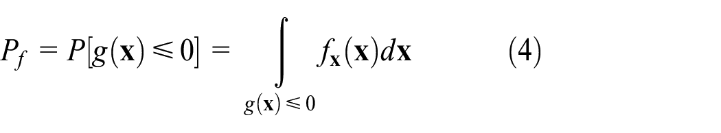
where f_x(x) is the joint probability density function (PDF) of x.

Although it is impractical to calculate the failure probability P_f using the multi-dimensional integration shown in equation (4), FORM allows us to calculate the probability analytically, by solving a constrained optimization problem.

In addition, FORM enables sensitivity analysis to evaluate the effects of the RVs on the failure probability, and it facilitates effective risk management by finding the most critical variable for reducing the risk. The sensitivity analysis provides not only quantitative measures for determining the importance of variables but also gradient-based optimizers for structural optimization.³³ FORM provides not only the component failure probability but also the component sensitivity, that is, the influence of the RVs on the component failure probability.

Each RV and the associated probability have different scales, and this affects the scale of the sensitivity. Therefore, the sensitivity of each RV should be normalized to assess its contribution to structural failure. The normalized sensitivity is simply the product of the non-normalized sensitivity and the standard deviation of an RV, as follows

δ_{i} = \frac{\partial P_{f}}{\partial μ_{i}} σ_{i}

(5a)

η_{i} = \frac{\partial P_{f}}{\partial σ_{i}} σ_{i}

(5b)

where δ_i and η_i denote the normalized probability sensitivities of the mean and standard deviation of the ith design variable, respectively. These normalized sensitivities provide information for design optimization, quality control, and uncertainty management.

In this study, FERUM is selected for the reliability analysis. FERUM is a reliability analysis package developed by researchers from the University of California at Berkeley to perform various reliability analyses.³⁴ FERUM offers functions of various reliability analysis methods including FORM, second-order reliability method (SORM), MCS, and importance sampling simulation, and most of the common probability distribution types are available for the program. In addition, the source codes of the program are open to the public (http://projects.ce.berkeley.edu/ferum). In addition, FERUM is built in MATLAB, which facilitates the reliability analysis via the response surface function obtained using MATLAB-ABAQUS.

Illustrative example: steel plate

Finite element analysis

As an illustrative example, the proposed framework is applied to a steel plate. As shown in Figure 2 (left), the steel plate has a width of 100 mm and a length of 200 mm, and an initial crack with a length of 0.1 mm is assumed on the left side of the center. The crack assumed at the center propagates under the application of a point load at the top left of the plate, ultimately leading to the fracture failure of the steel plate. As shown in Figure 2 (right), a finite element model is constructed for ABAQUS. The steel plate is modeled with shell elements, and cohesive elements are introduced along the centerline to simulate crack propagation. It is assumed that this model would exhibit elastic and geometrically nonlinear behavior. Finally, this model is controlled in terms of the displacement at the left-upper point for a better convergence of solutions.

Figure 2.

Illustrative example (left) and its ABAQUS model (right).

To model the numerical example of this study for ABAQUS, the CPS4R element, which is a four-node bilinear element with reduced integration, is used for the steel plate, and the COH2D4 element, which is a four-node 2D cohesive element, is used for the potential cracking zone. The traction-separation-based modeling is employed, and using the QUADS criterion, damage is assumed to initiate when a quadratic interaction function involving the nominal stress ratios reaches a value of 1, which can be expressed by

{\frac{t_{n}}{t_{n}^{0}}}^{2} + {\frac{t_{s}}{t_{s}^{0}}}^{2} = 1

(6)

where t_n and t_s denote the normal and shear tractions, respectively, and $t_{n}^{0}$ and $t_{s}^{0}$ denote their respective peak values. In this example, $t_{n}^{0}$ and $t_{s}^{0}$ are assumed to be 450 and 260 MPa, respectively.

Once the damage is initiated, it evolves, which eventually leads to failure at the bonded interface when the damage reaches a certain level. In this example, the evolution of damage is estimated in terms of energy using the following equation

{\frac{G_{n}}{G_{IC}}}^{2} + {\frac{G_{s}}{G_{IIC}}}^{2} = 1

(7)

where G_n and G_s denote the cohesive energies in normal and shear, respectively, and G_IC and G_IIC denote their threshold values. In this example, G_IC and G_IIC are assumed to be 50 and 20 kJ/m², respectively.

Table 2 lists the statistical properties (i.e. mean, standard deviation, and distribution type) of the RVs, all of which are material properties. As it is an illustrative example, for the sake of simplicity, it is also assumed that the RVs are statistically independent normal variates. However, if appropriate experimental data are available, other types of probability distributions and non-zero correlation coefficients can be introduced into the reliability analysis using FERUM, and such a parametric study is also conducted in this research.

Table 2.

Statistical properties of the RVs.

RV	Mean	Standard deviation	Distribution type
Young’s modulus (E)	2 × 10⁵ MPa	1 × 10⁴ MPa	Normal
Shear modulus (G)	8 × 10⁴ MPa	4 × 10³ MPa
Poisson’s ratio (ν)	0.3	0.015
Cohesive energy in tension (G_IC)	50 kJ/m²	2.5 kJ/m²
Cohesive energy in shear (G_IIC)	20 kJ/m²	1 kJ/m²
Tensile strength (S_{u_tensile})	450 MPa	9 MPa
Shear strength (S_{u_shear})	260 MPa	5.2 MPa

RV: random variable.

Figure 3 shows the stress distribution and crack propagation from the finite element analysis with the mean values of the seven RVs. As shown in the figure, the cohesive elements are continuously eliminated, and the stress is concentrated around the cracking zone as the crack propagates.

Figure 3.

Finite element analysis results using mean values of RVs.

In addition, Figure 4 shows the force–displacement plot at the loading point. The force stops increasing at a critical point and decreases until failure. When employing the mean values of the RVs, the maximum force and the corresponding displacement are found to be 1.594 × 10³ N and 2.676 × 10⁻¹ mm, respectively.

Figure 4.

Force–displacement curve.

Regarding this finite element analysis, it should be noted that each analysis takes approximately 1–2 h (using a general personal computer with 3.60 GHz CPU and 8.00 GB of RAM). Several approaches have been developed to perform reliability analysis in conjunction with finite element analysis.^35–40 However, such an approach requires performing finite element analysis repeatedly, which makes the analysis expensive and impractical. To overcome this issue, the RSM is introduced in the framework proposed in this article, in which the response surface function can be identified by performing only a few iterations of finite element analysis.

Response surface construction

To construct a response surface, as mentioned in section “Response surface construction,” the RV values in equation (2a) or (2b) need to be determined. They are often determined by adding to or subtracting from the mean a certain multiple of the standard deviation. In this illustrative example, for each RV, two times the standard deviation is added to or subtracted from the mean. A finite element analysis is then performed with these values. Table 3 lists the corresponding FE analysis results obtained from ABAQUS. In the table, for example, DOE No. 1 is the case with the mean values of all the RVs. In Nos 2 and 3, compared to No. 1, only Young’s modulus (E) is changed; twice the standard deviation (i.e. 2 × 1 × 10⁴ MPa) is added to and subtracted from the mean, respectively. Similarly, the other DOEs (i.e. Nos 4–15) can be determined.

Table 3.

Finite element analysis results for response surface construction.

DOE no.	E (MPa)	G (MPa)	v	G_IC (kJ/m²)	G_IIC (kJ/m²)	S_{u_tensile} (MPa)	S_{u_shear} (MPa)	P_c (N)	u_c (mm)
1	2.0 × 10⁵	8.0 × 10⁴	0.3	50	20	450	260	1594.49	0.269
2	1.8 × 10⁵	8.0 × 10⁴	0.3	50	20	450	260	1576.56	0.288
3	2.2 × 10⁵	8.0 × 10⁴	0.3	50	20	450	260	1610.89	0.249
4	2.0 × 10⁵	7.2 × 10⁴	0.3	50	20	450	260	1594.61	0.268
5	2.0 × 10⁵	8.8 × 10⁴	0.3	50	20	450	260	1594.38	0.268
6	2.0 × 10⁵	8.0 × 10⁴	0.27	50	20	450	260	1594.2	0.268
7	2.0 × 10⁵	8.0 × 10⁴	0.33	50	20	450	260	1594.8	0.267
8	2.0 × 10⁵	8.0 × 10⁴	0.3	45	20	450	260	1573.1	0.257
9	2.0 × 10⁵	8.0 × 10⁴	0.3	55	20	450	260	1614.13	0.269
10	2.0 × 10⁵	8.0 × 10⁴	0.3	50	18	450	260	1594.46	0.268
11	2.0 × 10⁵	8.0 × 10⁴	0.3	50	22	450	260	1594.52	0.268
12	2.0 × 10⁵	8.0 × 10⁴	0.3	50	20	432	260	1545.18	0.264
13	2.0 × 10⁵	8.0 × 10⁴	0.3	50	20	468	260	1643.11	0.280
14	2.0 × 10⁵	8.0 × 10⁴	0.3	50	20	450	249.6	1594.1	0.267
15	2.0 × 10⁵	8.0 × 10⁴	0.3	50	20	450	270.4	1594.65	0.268

DOE: design of experiment.

The finite analysis results, listed in Table 3, demonstrate that the effects of changes in shear modulus (G), Poisson’s ratio (ν), cohesive energy in shear (G_IIC), and shear strength (S_{u_shear}) on the critical force and displacement are largely insignificant. It is known that the error of the FORM analysis may increase as the number of RVs increases.⁴¹ In addition, reducing the number of RVs can result in a more efficient analysis. For these reasons, these four RVs are neglected in all further analyses.

With the remaining three RVs, that is, Young’s modulus (E), cohesive energy in tension (G_IC), and tensile strength (S_{u_tensile}), additional DOEs are determined, and a finite element analysis is then performed to construct the CCD response function with better accuracy. For the additional DOEs, all the combinations of the “mean ± 2 standard deviation” are considered for the three dominant RVs, whereas only the mean values are used for the other RVs. Table 4 lists the corresponding analysis results.

Table 4.

Additional results of finite element analysis for CCD response function.

DOE no.	E (MPa)	G (MPa)	v	G_IC (kJ/m²)	G_IIC (kJ/m²)	S_{u_tensile} (MPa)	S_{u_shear} (MPa)	P_c (N)	u_c (mm)
16	1.8 × 10⁵	8.0 × 10⁴	0.3	45	20	432	260	1507.45	0.273
17	1.8 × 10⁵	8.0 × 10⁴	0.3	45	20	468	260	1601.39	0.281
18	1.8 × 10⁵	8.0 × 10⁴	0.3	55	20	432	260	1547.42	0.285
19	1.8 × 10⁵	8.0 × 10⁴	0.3	55	20	468	260	1645.23	0.293
20	2.2 × 10⁵	8.0 × 10⁴	0.3	45	20	432	260	1540.58	0.236
21	2.2 × 10⁵	8.0 × 10⁴	0.3	45	20	468	260	1637.77	0.242
22	2.2 × 10⁵	8.0 × 10⁴	0.3	55	20	432	260	1578.51	0.247
23	2.2 × 10⁵	8.0 × 10⁴	0.3	55	20	468	260	1679.67	0.254

CCD: central composite design; DOE: design of experiment.

Based on the finite analysis results listed in Tables 3 and 4, the response surface functions for the critical force (P_c) and displacement (u_c) are constructed as follows

\begin{matrix} P_{c} = - 70.24 + 9.416 \times 10^{- 4} E + 4.317 G_{IC} \\ + 2.979 S_{u_tensile} \\ - 4.975 \times 10^{- 6} E G_{IC} + 2.292 \times 10^{- 6} E S_{u_tensile} \\ + 0.01089 G_{IC} S_{u_tensile} \\ - 2.193 \times 10^{- 9} E^{2} - 0.03949 \times G_{IC}^{2} \\ - 0.001411 S_{u_tensile}^{2} \end{matrix}

(8a)

\begin{matrix} u_{c} = 0.9367 + 3.928 \times 10^{- 7} E + 0.02641 G_{IC} \\ - 0.006026 S_{u_tensile} \\ - 1.641 \times 10^{- 9} E G_{IC} - 7.06 \times 10^{- 10} E S_{u_tensile} \\ + 7.069 \times 10^{- 7} G_{IC} S_{u_tensile} \\ - 2.387 \times 10^{- 12} E^{2} - 2.522 \times 10^{- 4} \times G_{IC}^{2} \\ + 7.087 \times 10^{- 6} S_{u_tensile}^{2} \end{matrix}

(8b)

To analyze the approximation error of the response surface functions, the function values are compared with the true values obtained from finite element analyses for all DOEs. As shown in Table 5, the maximum values of absolute error ratios are calculated to be 0.048% and 1.274% for P_c and u_c, respectively, which means that the response surface functions in equations (8a) and (8b) can provide good approximations of P_c and u_c.

Table 5.

Error analysis of the response surface functions.

DOE no.	P_c			u_c
DOE no.	FEA (N)	RSM (N)	Absolute error ratio (%)	FEA (mm)	RSM (mm)	Absolute error ratio (%)
1	1594.49	1594.86	0.023	0.269	0.269	0
2	1576.56	1577.04	0.03	0.288	0.287	0.347
3	1610.89	1610.93	0.002	0.249	0.249	0
4	1594.61	1594.86	0.016	0.268	0.269	0.373
5	1594.38	1594.86	0.03	0.268	0.269	0.373
6	1594.2	1594.86	0.041	0.268	0.269	0.373
7	1594.8	1594.86	0.004	0.267	0.269	0.749
8	1573.1	1573.41	0.02	0.257	0.257	0
9	1614.13	1614.34	0.013	0.269	0.269	0
10	1594.46	1594.86	0.025	0.268	0.269	0.373
11	1594.52	1594.86	0.021	0.268	0.269	0.373
12	1545.18	1545.59	0.027	0.264	0.267	1.136
13	1643.11	1643.22	0.007	0.280	0.276	1.429
14	1594.1	1594.86	0.048	0.267	0.269	0.749
15	1594.65	1594.86	0.013	0.268	0.269	0.373
16	1507.45	1507.62	0.011	0.273	0.273	0
17	1601.39	1601.65	0.016	0.281	0.282	0.356
18	1547.42	1547.59	0.011	0.285	0.285	0
19	1645.23	1645.54	0.019	0.293	0.294	0.341
20	1540.58	1540.85	0.018	0.236	0.235	0.424
21	1637.77	1638.17	0.024	0.242	0.243	0.413
22	1578.51	1578.83	0.02	0.247	0.246	0.405
23	1679.67	1680.07	0.024	0.254	0.255	0.394

DOE: design of experiment; FEA: finite element analysis; RSM: response surface method.

Risk and sensitivity quantification results

Using the response surface functions expressed in equations (6a) and (6b), the FORM analysis is performed by FERUM. The first available result is the uncertainty quantification of the output, that is, P_c and u_c, in terms of the PDF and cumulative density function (CDF), as shown in Figures 5 and 6. The figures show the probabilistic distribution of the uncertain outputs induced by the input uncertainties.

Figure 5.

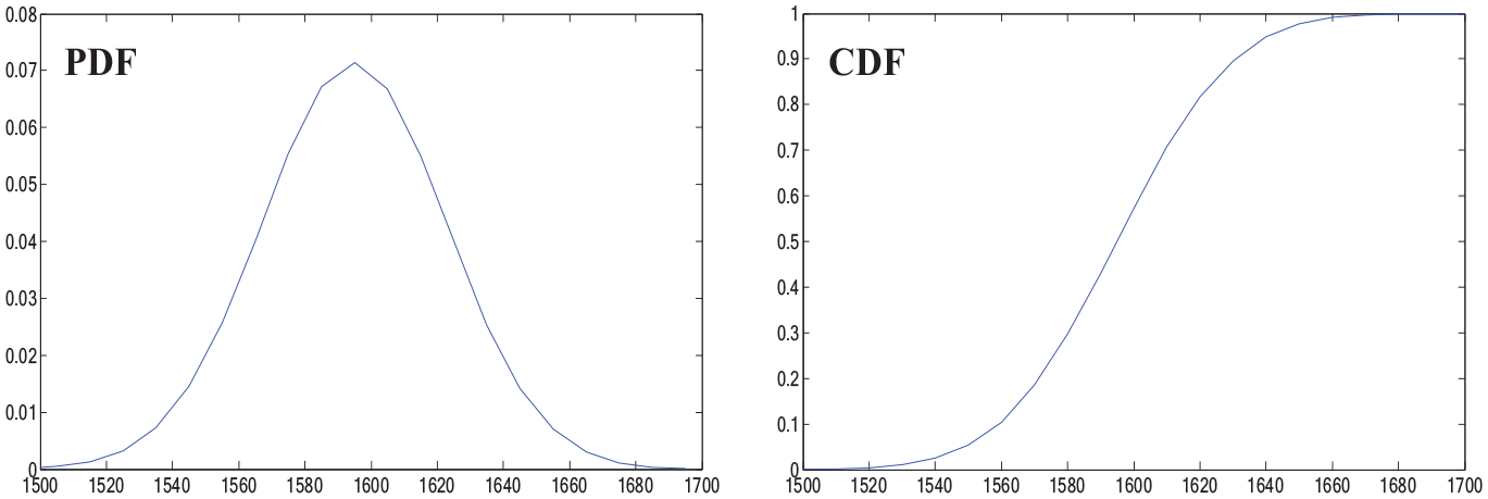
PDF and CDF of P_c.

Figure 6.

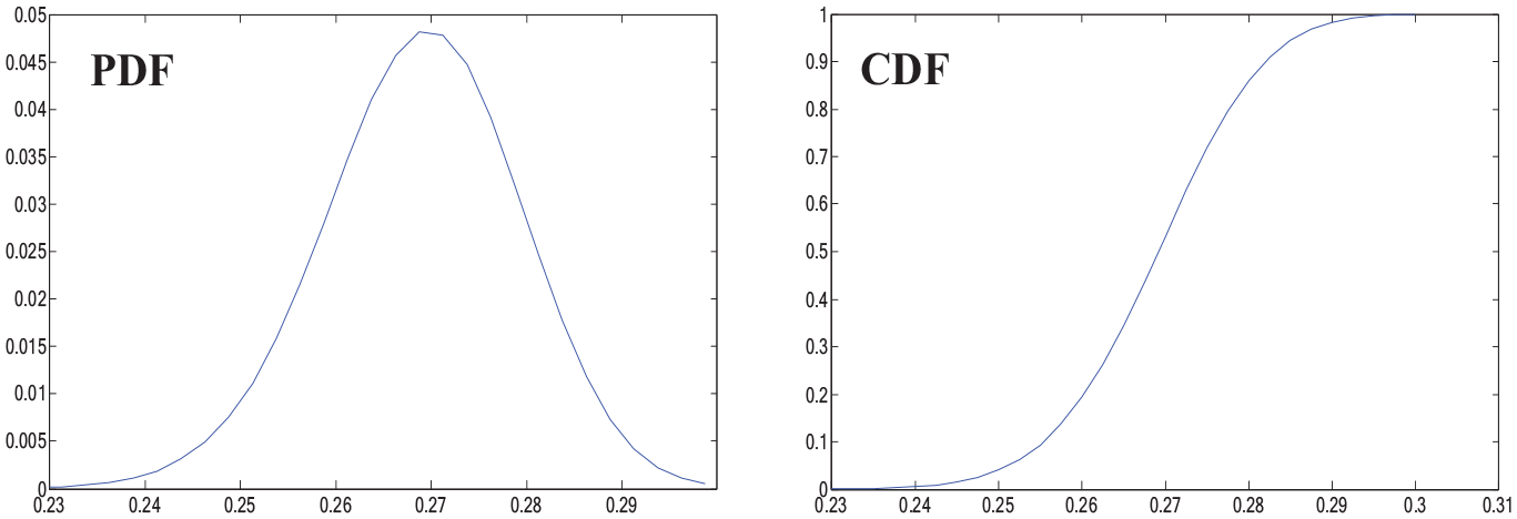
PDF and CDF of u_c.

Another result of the reliability analysis is risk quantification, which can be obtained by evaluating a failure probability for a given limit-state function. For example, the probability of P_c being lower than 1530 N (i.e. P_c − 1530 < 0 named E₁ hereafter) is calculated to be 0.991% from the FORM analysis. Similarly, the probability of u_c being greater than 0.290 mm (i.e. 0.29 − u_c < 0 named E₂ hereafter) is calculated to be 1.690%. To verify these FORM analysis results, MCS with 10⁶ samples is performed, and the failure probabilities are estimated to be 1.013% and 1.685% for E₁ and E₂, respectively, which shows a good agreement with the FORM analysis. In addition, when all of the RVs are assumed to follow the lognormal distributions with the same statistical parameters (i.e. the means and standard deviations given in Table 2), the probabilities are estimated to be 0.930% and 1.398% for E₁ and E₂, respectively, which shows only a certain degree of change, but not a dramatic change.

In addition to such failure probabilities, using equations (5a) and (5b), FORM can provide the normalized sensitivity of the probability with respect to the statistical parameters of RVs, and these results are presented in Table 6. S_{u_tensile} and E are observed to be the most important RVs for E₁ and E₂, respectively (from Table 6). All of the three RVs exhibit negative probability sensitivities for E₁ with respect to their mean values, which means that the failure probabilities of E₁ decrease with increasing mean values. In contrast, for E₂, E exhibits a negative sensitivity, but G_IC and S_{u_tensile} exhibit positive sensitivities, which means the failure probabilities of E₂ decrease with the increasing mean values of E and the decreasing mean values of G_IC and S_{u_tensile}. Finally, for the probabilities of both E₁ and E₂, all of the RVs exhibit positive sensitivities with respect to their standard deviations.

Table 6.

Normalized sensitivity of probability with respect to the statistical parameters of RVs.

RVs	E ₁: P_c − 1530 < 0		E ₂: 0.29 − u_c < 0
RVs	$δ_{i} = \frac{\partial P_{f}}{\partial μ_{i}} σ_{i}$	$η_{i} = \frac{\partial P_{f}}{\partial σ_{i}} σ_{i}$	$δ_{i} = \frac{\partial P_{f}}{\partial μ_{i}} σ_{i}$	$η_{i} = \frac{\partial P_{f}}{\partial σ_{i}} σ_{i}$
Young’s modulus (E)	−8.02 × 10⁻³	5.67 × 10⁻³	−3.87 × 10⁻²	7.6 × 10⁻²
Cohesive energy in tension (G_IC)	−9.71 × 10⁻³	8.31 × 10⁻³	7.9 × 10⁻³	3.15 × 10⁻³
Tensile strength (S_{u_tensile})	−2.32 × 10⁻³	4.76 × 10⁻²	1.4 × 10⁻²	9.94 × 10⁻³

RV: random variable.

In addition, to investigate the effect of statistical dependence between random variables on the failure probabilities for E₁ and E₂, the FORM analysis is performed with varying correlation coefficients between the three assumed RVs (i.e. Young’s modulus (E), cohesive energy in tension (G_IC), and tensile strength (S_{u_tensile})). As shown in Table 7, with the increasing correlation coefficient, the probability of E₁ increases but the probability of E₂ decreases.

Table 7.

Parametric study on the effect of correlation between RVs.

Correlationcoefficient	Probability (%)
Correlationcoefficient	E ₁: P_c − 1530 < 0	E ₂: 0.29 − u_c < 0
0	0.991	1.69
0.2	1.986	0.996
0.4	3.151	0.448
0.6	4.377	0.11
0.8	5.602	0.03

RV: random variable.

Using FORM, it is also possible to estimate the contributions of the input uncertainties to the output uncertainties in terms of the importance measure. The importance measure is a normalized relative measure to 100%, representing the importance of the uncertainty of an RV with respect to the variance of the output uncertainty. In other words, the higher the importance measure, the higher is the degree of contribution. Table 8 lists the results.

Table 8.

Importance of dominant RVs to E₁ and E₂.

RVs	Importanceto E₁ (%)	Importanceto E₂ (%)
E	9.2	85.3
G_IC	13.4	3.5
S_{u_tensile}	77.4	11.2

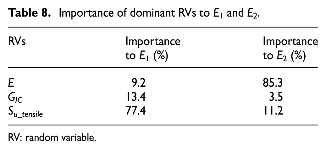
RV: random variable.

From this table, it is confirmed that the tensile stress (S_{u_tensile}) is the most important RV with respect to E₁, whereas Young’s modulus (E) is the most important RV with respect to E₂. The reliability analysis results are understandable because it is known that the ultimate tensile stress governs the strength of a steel plate in mode I. However, in the case of the critical displacement, it would be Young’s modulus. In this manner, the proposed framework enables the quantitative evaluation of the relative importance of RVs efficiently.

Conclusion

This article proposes a new probabilistic framework for the risk and sensitivity analysis of structural fatigue failure employing CZEs. The proposed framework comprises three steps, namely finite element analysis using CZEs, response surface construction, and risk and sensitivity analyses of fatigue failure, which require several mathematical techniques. The proposed framework was illustrated by applying it to a numerical example, and the analysis results of fatigue failure probability with different threshold values of a limit-state function were obtained. In addition, the normalized sensitivity of failure risk with respect to the statistical parameters of each random variable was presented and discussed. The proposed framework allows quantifying the output uncertainties and risk for any limit-state function, and the failure probability results were compared with those from MCS. In addition, the framework helps compare the relative importance of the inputs in terms of their contribution to the output uncertainties. An illustrative example of a steel plate cracking problem was introduced to demonstrate the applicability of the proposed framework, and the corresponding analysis results proved the merits of the proposed framework employing cohesive zone modeling successfully.

Footnotes

Handling Editor: James Baldwin

Declaration of conflicting interests

The author(s) declared no potential conflicts of interest with respect to the research, authorship, and/or publication of this article.

Funding

The author(s) disclosed receipt of the following financial support for the research, authorship, and/or publication of this article: This work was supported by the 2019 Research Fund (1.190047.01) of Ulsan National Institute of Science and Technology (UNIST). This study was also supported by a grant (19POQW-B152755-01) from the Transportation Logistics Research Program funded by the Ministry of Land, Infrastructure and Transport (MOLIT) of the Korean government and the Korea Agency for Infrastructure Technology Advancement (KAIA).

ORCID iD

Wonho Suh

References

Lee

Cho

. SHM-based probabilistic fatigue life prediction for bridges based on FE model updating. Sensors 2016; 16: 317.

Suresh

. Fatigue of materials. Cambridge: Cambridge University Press, 1998.

Stephens

Fatemi

Stephens

, et al. Metal fatigue in engineering. New York: John Wiley & Sons, 2000.

Lee

Kim

Suh

, et al. Probabilistic fatigue life updating for railway bridges based on local inspection and repair. Sensors 2017; 17: 936.

Schijve

. Fatigue predictions and scatter. Fatigue Fract Eng Mater Struct 1994; 17: 381–396.

Paris

Erdogan

. A critical analysis of crack propagation laws. J Basic Eng 1963; 85: 528–533.

Zhao

Haldar

Breen

. Fatigue-reliability evaluation of steel bridges. J Struct Eng 1994; 120: 1608–1623.

Lee

Song

. Finite-element-based system reliability analysis of fatigue-induced sequential failures. Reliabil Eng Syst Safety 2012; 108: 131–141.

Soares

Garbatov

. Fatigue reliability of the ship hull girder accounting for inspection and repair. Reliabil Eng Syst Safety 1996; 51: 341–351.

10.

Karamchandani

Dalane

Bjerager

. Systems reliability approach to fatigue of structures. J Struct Eng 1992; 118: 684–700.

11.

Moan

Song

. Implications of inspection updating on system fatigue reliability of offshore structures. J Offshore Mech Arctic Eng 2000; 122: 173–180.

12.

Sørensen

. Framework for risk-based planning of operation and maintenance for offshore wind turbines. Wind Energy 2009; 12: 493–506.

13.

Dowling

Calhoun

Arcari

. Mean stress effects in stress-life fatigue and the Walker equation. Fatigue Fract Eng Mater Struct 2009; 32: 163–179.

14.

Klesnil

Lukáš

. Influence of strength and stress history on growth and stabilisation of fatigue cracks. Eng Fract Mech 1972; 4: 77–92.

15.

Donahue

Clark

Atanmo

, et al. Crack opening displacement and the rate of fatigue crack growth. Int J Fract Mech 1972; 8: 209–219.

16.

Dugdale

. Yielding of steel sheets containing slits. J Mech Phys Solids 1960; 8: 100–104.

17.

Barenblatt

. The mathematical theory of equilibrium cracks in brittle fracture. Adv Appl Mech 1962; 7: 55–129.

18.

Hariri-Ardebili

Saouma

. Sensitivity and uncertainty quantification of the cohesive crack model. Eng Fract Mech 2016; 155: 18–35.

19.

Beaurepaire

Schuëller

. Modeling of the variability of fatigue crack growth using cohesive zone elements. Eng Fract Mech 2011; 78: 2399–2413.

20.

Wang

Atluri

. Recent advances in the alternating method for elastic and inelastic fracture analyses. Comp Meth Appl Mech Eng 1996; 137: 1–58.

21.

Moës

Dolbow

Belytschko

. A finite element method for crack growth without remeshing. Int J Numer Meth Eng 1999; 46: 131–150.

22.

Valdebenito

Schuëller

. Design of maintenance schedules for fatigue-prone metallic components using reliability-based optimization. Comp Meth Appl Mech Eng 2010; 199: 2305–2318.

23.

Song

Budyn

, et al. A method for growing multiple cracks without remeshing and its application to fatigue crack growth. Model Simulat Mater Sci Eng 2004; 12: 901.

24.

De Borst

Remmers

Needleman

. Mesh-independent discrete numerical representations of cohesive-zone models. Eng Fract Mech 2006; 73: 160–177.

25.

Nguyen

Repetto

Ortiz

, et al. A cohesive model of fatigue crack growth. Int J Fract 2001; 110: 351–369.

26.

Hillerborg

Modéer

Petersson

. Analysis of crack formation and crack growth in concrete by means of fracture mechanics and finite elements. Cement Concrete Res 1976; 6: 773–781.

27.

Dassault Systèmes. Abaqus analysis user’s manual. Providence, RI: Simulia Corp, 2007.

28.

Bucher

Bourgund

. Efficient use of response surface methods. Innsbruck: Institut für Mechanik, Universität Innsbruck, 1987

29.

Myers

. Response surface methodology. Boston, MA: Allyn & Bacon, 1971.

30.

Haldar

. Recent developments in reliability-based civil engineering. Singapore: World Scientific Publishing Company, 2006.

31.

Melchers

. Structural reliability: analysis and prediction. 2nd ed. New York: John Wiley & Sons, 1999.

32.

Der Kiureghian

. First- and second-order reliability methods (Chapter 14). In: Nikolaidis

Ghiocel

Singhal

(eds) Engineering design reliability handbook. Boca Raton, FL: CRC Press, 2005, pp.14-1–14-24.

33.

Chun

Song

Paulino

. Parameter sensitivity of system reliability using sequential compounding method. Struct Safety 2015; 55: 26–36.

34.

Haukaas

. Finite element reliability and sensitivity methods for performance-based engineering, vol. 1. Berkeley, CA: University of California, 2003.

35.

Lee

Kim

, et al. A new methodology development for flood fragility curve derivation considering structural deterioration for bridges. Smart Struct Syst 2016; 17: 149–165.

36.

Lee

Moon

. A new methodology of the development of seismic fragility curves. Smart Struct Syst 2014; 14: 847–867.

37.

Lee

Song

. System reliability updating of fatigue-induced sequential failures. J Struct Eng 2014; 140: 04013074.

38.

Lee

Song

Tuegel

. Finite element system reliability analysis of a wing torque box. In: 10th AIAA non-deterministic approaches conference, 7–10 April 2008, Schaumburg, IL. Reston, VA: AIAA.

39.

Kang

Lee

Song

, et al. Further development of matrix-based system reliability method and applications to structural systems. Struct Infrastruct Eng 2012; 8: 441–457.

40.

Kim

Sim

Lee

, et al. Flood fragility analysis for bridges with multiple failure modes. Adv Mech Eng. Epub ahead of print 17 March 2017. DOI: 10.1177/1687814017696415.

41.

Miller

Baker

Lim

, et al. A FORM-based analysis of lifeline networks using a multivariate seismic intensity model. In: 11th international conference on applications of statistics and probability in civil engineering (ICASP11), 1–4 August 2011 Boca Raton, FL: CRC Press.

Risk and sensitivity quantification of fracture failure employing cohesive zone elements

Abstract

Keywords

Introduction

Proposed framework

Finite element analysis employing CZEs

Response surface construction

Risk and sensitivity quantification

Illustrative example: steel plate

Finite element analysis

Response surface construction

Risk and sensitivity quantification results

Conclusion

Footnotes

Declaration of conflicting interests

Funding

ORCID iD

References