
Abstract
A new fault detection technique is considered in this article. It is based on kernel partial least squares, exponentially weighted moving average, and generalized likelihood ratio test. The developed approach aims to improve monitoring the structural systems. It consists of computing an optimal statistic that merges the current information and the previous one and gives more weight to the most recent information. To improve the performances of the developed kernel partial least squares model even further, multiscale representation of data will be used to develop a multiscale extension of this method. Multiscale representation is a powerful data analysis way that presents efficient separation of deterministic characteristics from random noise. Thus, multiscale kernel partial least squares method that combines the advantages of the kernel partial least squares method with those of multiscale representation will be developed to enhance the structural modeling performance. The effectiveness of the proposed approach is assessed using two examples: synthetic data and benchmark structure. The simulation study proves the efficiency of the developed technique over the classical detection approaches in terms of false alarm rate, missed detection rate, and detection speed.
Keywords
Introduction
Structural health monitoring (SHM) is considered as an approach to monitor the structure systems. It consists of developing monitoring solutions based on the data collected by the sensors installed on the structure. Its purpose is to detect, identify, estimate, and/or locate the existing faults on the structure and to make decisions concerning its evolution and its state in order to improve its safety. In the current work, we will focus on the fault detection (FD) problem.
In the literature, many methods for detecting faults1–3 have been considered. They can be defined as methods based on a model4–6 or as data-driven methods.7–12 Many physical systems of the actual civil structure are complex and difficult to construct their models.13,14 Therefore, data-driven methods are widely used for monitoring and FD purposes. 15
Latent variable regression (LVR) is a well-known data-driven modeling technique that includes principal component analysis (PCA) 16 and partial least squares (PLS). 17 LVR modeling methods are a multivariate analysis that aims to reduce the dimensionality of the data and rely on the definition of a linear data transformation via an orthonormal matrix which is computed from the dataset itself.
However, most of the practical systems are input–output, nonlinear, and multivariate. To make the extension to input–output, nonlinear, and multivariate models, kernel partial least squares (KPLS) will be used for the modeling purposes. The benefits of using the KPLS model lie in the fact that it does not require nonlinear optimization and it only requires the solution of an eigenvalue problem.
To improve the performances of the KPLS model even further, multiscale representation of data will be used to develop a multiscale kernel partial least squares (MSKPLS) method. Multiscale representation is a powerful data analysis way that presents efficient separation of deterministic characteristics from random noise.
Once the model is built, the monitoring technique should be addressed in order to detect the faults in SHM systems. To do that, a novel detection chart based on generalized likelihood ratio test (GLRT) and exponentially weighted moving average (EWMA) chart statistics will be applied. The EWMA-GLRT chart depends upon evaluating the residuals, which are obtained from the MSKPLS to detect the fault in the network.
The benefits of the proposed EWMA-GLRT are to develop a new detection statistic that considers the current information and the previous one and strengthens the more recent information by providing more weight to it. Therefore, the developed FD technique consists of considering the MSKPLS for modeling purposes and EWMA-GLRT chart for detection and monitoring goals. The developed technique will be evaluated and compared to many other techniques using two examples: synthetic data and benchmark structure. The results show the efficiency of the proposed technique over the classical approaches in terms of false alarm rate (FAR), missed detection rate (MDR), and detection speed.
The rest of this article is arranged as follows: first, we describe the multiscale KPLS method in section “Multiscale KPLS description.” In section “OEWMA-GLRT detection chart description,” we present the new EWMA-GLRT chart. In section “Applications,” the effectiveness of the proposed approach is evaluated through synthetic data and a simulated SHM benchmarking data. Finally, we present the conclusions in section “Conclusion.”
Multiscale KPLS description
KPLS
Given an input matrix

where
Note that the matrices X and Y are first standardized to have zero mean and unit variance before constructing the PLS model. PLS assumes linear correlation among variables, which lead to prediction and modeling errors in cases of nonlinear processes. To address this issue and in order to extend this technique to deal with nonlinear input–output models, many extensions have been proposed to define the nonlinearities. The PLS has been extended to nonlinear regression through the use of kernel-based functions. The most well-known approach is called KPLS, which will be considered in the next section.
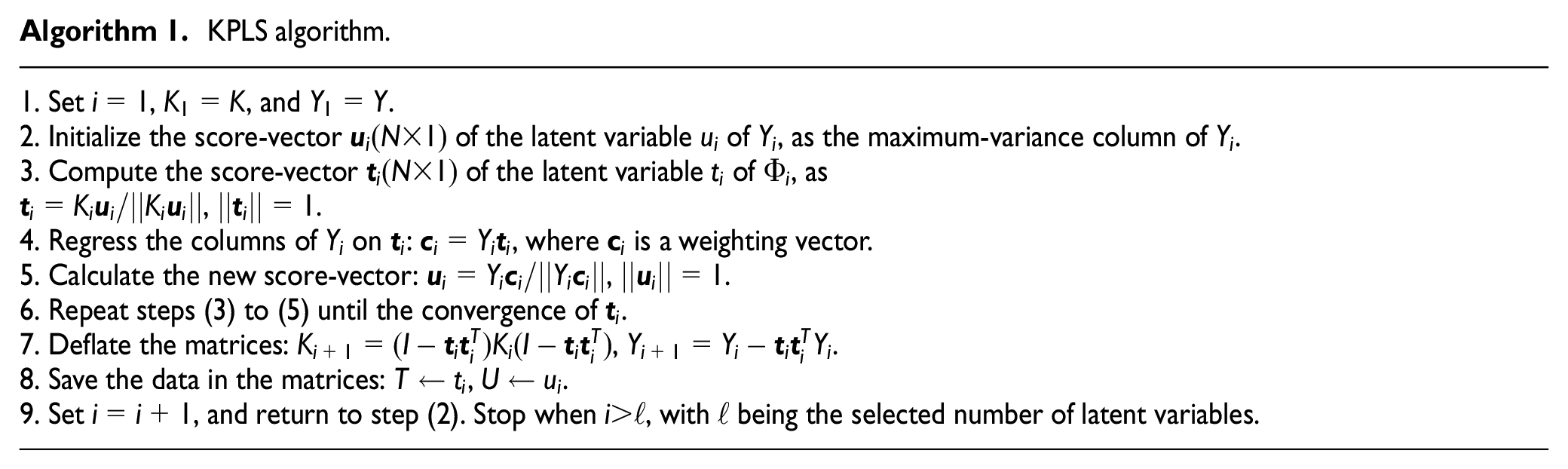
KPLS model
The KPLS method consists of using the classical PLS directly in the feature space. Its idea first is to map the original nonlinear data into a linear high-dimensional feature space and then to perform linear PLS in the feature space. The main idea of KPLS method is illustrated in Figure 1.

Basic idea of KPLS.
Define

where the dimension f can be arbitrarily large or even infinite.
In the feature space,

where

with
Thus, the zero mean of
According to Sheriff et al.,
19
the KPLS model of

where
Note that

where the entry

Thus, the kernel matrix K is given by
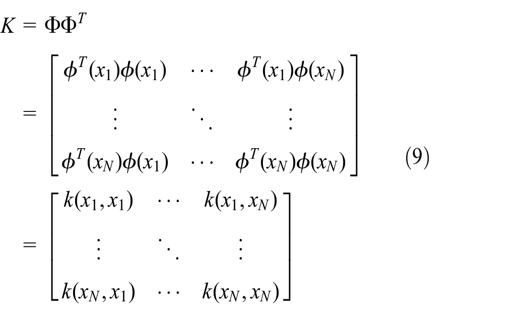
The function

where c is the width of a Gaussian function.
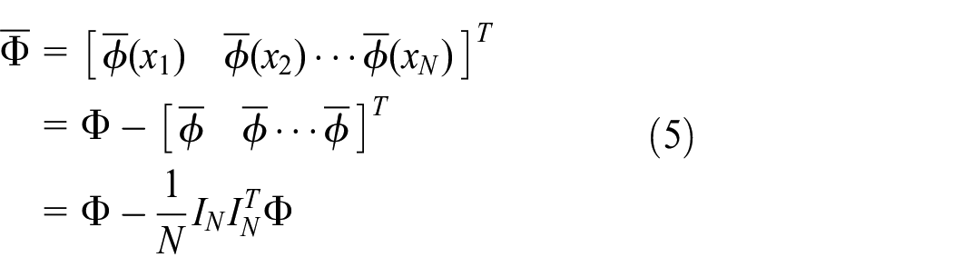
The kernel matrix K is centralized as

According to equation (5),
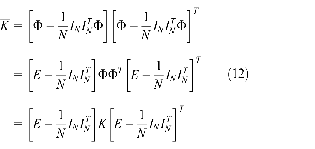
where I is the identity matrix.
From the centered data matrices K and Y, the regression coefficient matrix B can be obtained as22,23

The prediction of the response variables is given by

Equation (14) shows that the response variables (outputs) can be obtained from the inner products of the mapped vectors. Hence, for a new observation x of the predictor vector, the outputs are estimated by

where
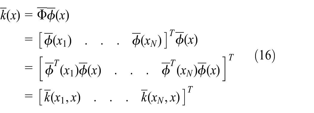
From equations (4), (5), and (16), the following relationships can be defined as

where
Multiscale KPLS technique
Teppola and Minkkinen 24 are the first who have developed the linear multiscale PLS, where the multiscale representation was combined with linear PLS model. It has been applied essentially to remove the drift in the data set. Zhang and Hu 25 have studied the nonlinear extension (MKPLS). The wavelet-based multiscale representation of data can ameliorate the KPLS modeling. Similar to the proposed method multiscale principal component analysis (MSPCA) by Bakshi and Top, 26 we shall use in this work the multiscale KPLS algorithm. Similar to PLS, the modeling using KPLS can be proceeded in the mapped feature space.
Given a data set of training data, the variables are decomposed in the feature space through the discrete wavelet transform (DWT). At each individual scale, KPLS model is applied. In order to construct the data, important scale coefficients are selected according to a statistical threshold (see Figure 2). Then, KPLS model is applied on global scale for FD. At each scale, the statistical thresholding is proceeded as a data filtering stage which improves KPLS efficiency. The MSKPLS algorithm is shown in Algorithm 2 and its representation model is shown in Figure 2.

Representation of MSKPLS model for FD.

Advantages of multiscale data representation
Multiscale representation has the ability to separate the noise from important features in the data. When data are decomposed at multiple scales by passing through low-pass and high-pass filters, noise is effectively separated from the important features. Random noise in a signal is normally present over all the coefficients, whereas deterministic features in the data are captured in a few but relatively large coefficients. The important features in the data are usually captured by the last scaled signals as well as any large wavelet coefficient (in the detail signals), whereas other small wavelet coefficients usually correspond to noise. 26 Thus, multiscale representation provides an effective method for noise-feature separation as shown in Figure 3.

A schematic diagram of data representation at multiple scales: (a) original signal, (b) first scaled signal, (c) first detail signal, (d) second scaled signal, (e) second detail signal, (f) third scaled signal, and (g) third detail signal. 26
The benefits of multiscale representation present that they can help verify the assumptions of independence, normality, and noise level made by several univariate and multivariate monitoring approaches. 27
The objective of the next section is to present MSKPLS-based optimized exponentially weighted moving average-generalized likelihood ratio test (OEWMA-GLRT) approach for FD purposes. The developed framework is addressed so that the modeling phase is addressed using the MSKPLS and the detection of the faults is achieved using the OEWMA-GLRT chart. The MSKPLS is used to compute the monitored residuals and the OEWMA-GLRT chart (which is presented next) is applied to the evaluated monitored residuals for FD purposes.
OEWMA-GLRT detection chart description
The new detection chart combines the advantages of the EWMA and GLRT charts. It also consists of optimizing the EWMA chart using a multi-objective function. It reduces the MDR, the FAR, and the detection speed
Classical GLRT detection chart
The GLRT chart is a commonly used hypothesis testing technique for FD in model-based methods.28,29 Let us denote for an observation vector
The parameter

where
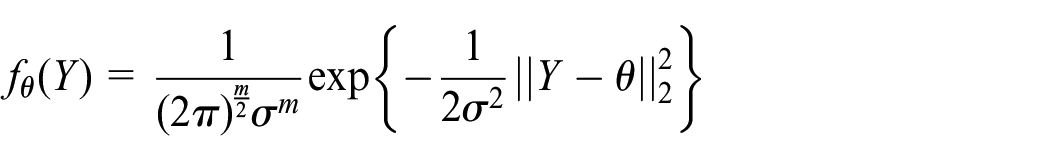
Note that the maximization of the likelihood function corresponds to the maximization of its logarithm. The distribution of the GLRT decision function

where

The GLRT technique is derived to detect a shift in the mean (fault), and its explicit asymptotic statistic is computed. It is used to detect an additive fault
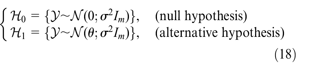
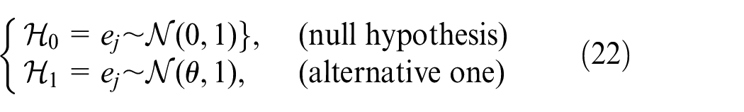
In this work, the FD problem is considered as a hypothesis test taking into account two possible hypotheses: a null hypothesis
From equation (18), let
and the GLRT statistic is presented as follows

In order to choose the threshold

If the GLRT statistic is the upper threshold
OEWMA-GLRT detection chart
The EWMA chart was first developed by Roberts 32 in 1959. It can be computed as follows 33

where
The EWMA chart has two control limits: an upper control limit
These control limits are computed as follows 34


where L represents the control width of the EWMA statistic Z and
In order to compute the optimal values
The OEWMA-GLRT statistic

where
In order to detect the faults in the residual vector R that is obtained from MSKPLS model, MSKPLS-based OEWMA-GLRT is proposed. The filtering and detection are two independent phases implemented in the FD algorithm (see Figure 4). Nevertheless, when these two tasks are simultaneously implemented, this may improve the FD abilities. Thus, we develop MSKPLS-based OEWMA-GLRT where the KPLS model is established based on the wavelet coefficients and the OEWMA-GLRT is applied to detect faults.
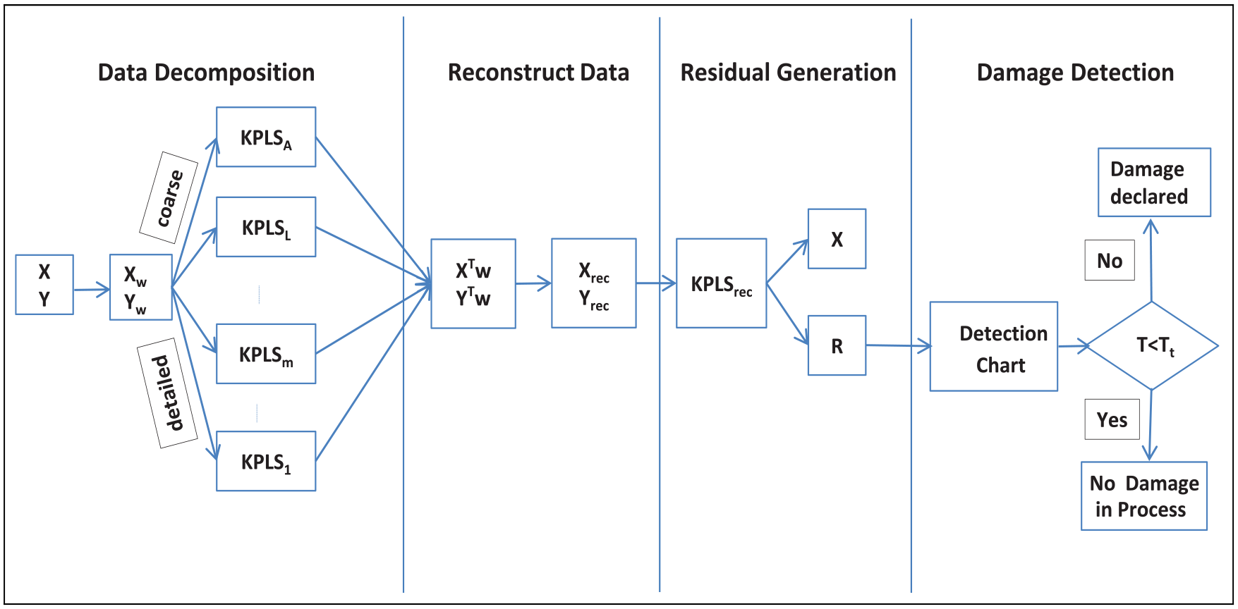
Schematic illustration of the developed MSKPLS-based OEWMA-GLRT approach.
The proposed MSKPLS-based OEWMA-GLRT technique for FD is described in Algorithm 3.

Applications
The validation of the developed approach is done through two simulated examples: synthetic data set 10 and benchmark model International Association for Structural Control-American Society of Civil Engineers (IASC-ASCE).36–39
FD using simulated example
The simulated example proposed in Bakshi 40 contains four variables where the first variable follows a normal distribution with zero mean and unit variance. The simulation is presented in the following equations

The input data matrix

The four model variables generated in the previous equation will be arranged in a matrix of the form

This matrix consists of four columns presenting the variables and
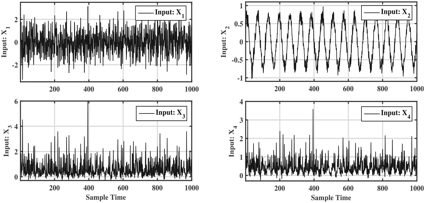
The time evolution of the input variables.
The output variable will be arranged in a data matrix Y and it is generated as the following equation

In order to construct the KPLS model, the input and output data should be scaled first. Then, the data set is divided into training data which consist of
To illustrate the performance of the proposed technique OEWMA-GLRT chart, we compare it with the other techniques such as the GLRT chart and the OEWMA chart. This comparison addresses the linear and the nonlinear cases processed by the PLS model and the KPLS model, respectively. In the KPLS model, the radial basis function (RBF) is used with a parameter

Results using PLS-based GLRT method.

Results using PLS-based OEWMA method.

Results using PLS-based OEWMA-GLRT method.

Results using KPLS-based GLRT method.

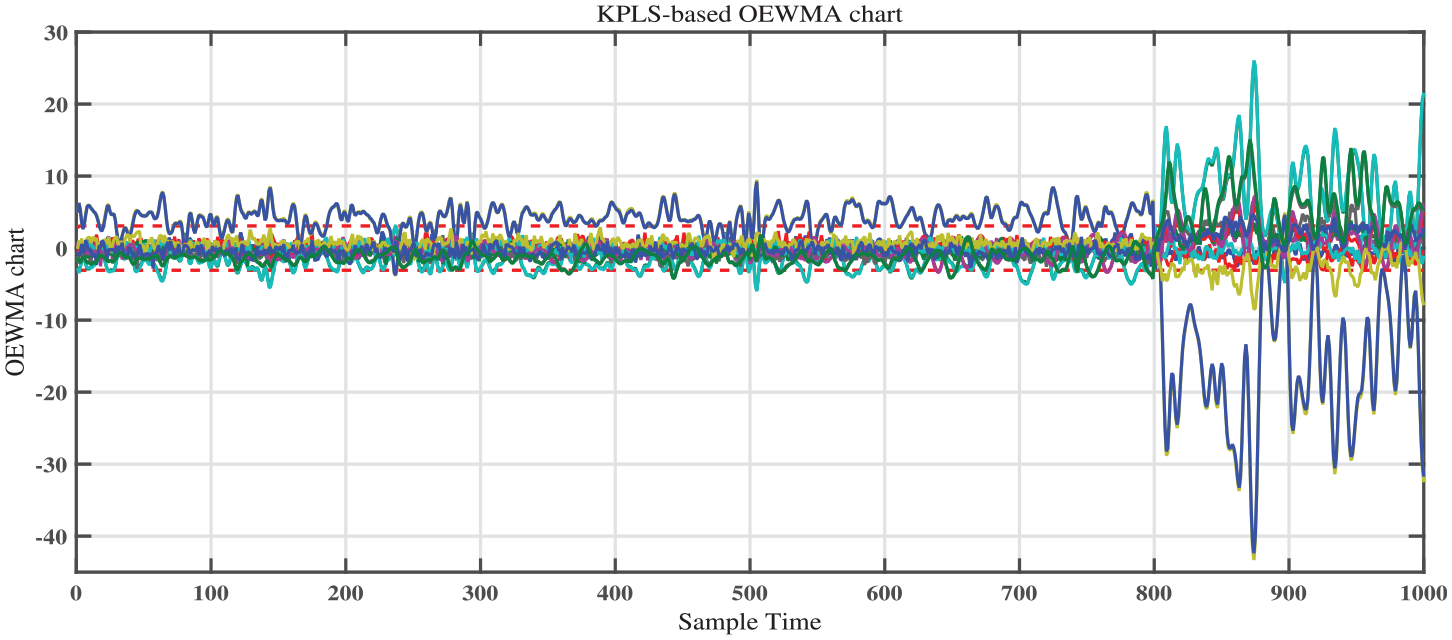
Results using KPLS-based OEWMA method.

Results using KPLS-based OEWMA-GLRT method.
Comparison in terms of MDR, FAR, and

GLRT: generalized likelihood ratio test; OEWMA: optimized exponentially weighted moving average; OEWMA-GLRT: optimized exponentially weighted moving average-generalized likelihood ratio test; MDR: missed detection rate; FAR: false alarm rate; PLS: partial least squares; KPLS: kernel partial least squares.
Figures 6–8 show that the PLS-based OEWMA-GLRT chart provides better detection results comparing to both PLS-based OEWMA and PLS-based GLRT charts. Otherwise, the results show that the detection abilities based on linear PLS model present a lot of false alarm and MDRs. This is because the PLS method assumes a linear relationship between variables. However, the simulated synthetic example (29) is nonlinear, which means that the linear PLS method cannot tackle the issue of non-linearity. To deal with this issue, KPLS method is applied here for modeling purposes. Figures 9–11 and Table 1 show the detection performances based on KPLS model. The benefits of KPLS model on the detection performances over the linear PLS model are shown in Table 1.
Figures 9–11 illustrate that the developed KPLS-based OEWMA-GLRT method gives the best detection quality with respect to the classical KPLS-based GLRT and KPLS-based OEWMA charts. All of them outperform the detection charts based on PLS model (see Figures 6–9). Table 1 illustrates this in terms of the detection metrics: MDR, FAR, and
Figures 12 and 13 and Table 2 show the effect of the multiscale representation on the detection abilities. In fact, the use of the multiscale representation of the data may enhance the monitoring quality by reducing the missed detection and the FARs. The wavelet-based multiscale representation of data may ameliorate the detection abilities of the KPLS- and PLS-based methods (Figures 8 and 11–13).

Results using MSPLS-based OEWMA-GLRT method.

Results using MSKPLS-based OEWMA-GLRT method.
Comparison in terms of MDR, FAR, and

MSPLS: multiscale partial least squares; MSKPLS: multiscale kernel partial least squares; MDR: missed detection rate; FAR: false alarm rate; OEWMA-GLRT: optimized exponentially weighted moving average-generalized likelihood ratio test.
FD using simulated benchmark process
The validation of the proposed approach is also assessed using a nonlinear simulated benchmark structure.36–39 The benchmark structures provided by the IASC-ASCE Structural Health Monitoring Group are studied to verify the effectiveness of damage detection.
The benchmark gives an analytical model based on the structure 12-degree-of-freedom (DOF) shear-building model. It consists of a
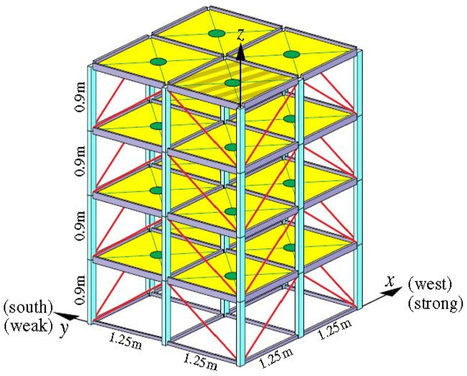
Steel frame scale structure.
More details on the IASC-ASCE benchmark are presented in Chaabane et al. 42 This model was developed to generate simulated input–output response data. 42
In order to construct the KPLS model, the input and output data should be scaled first. Then, the data set is divided into training data which consists of
When we apply the multiscale KPLS to construct the model, the best decomposition depth needs to be chosen in order to get good detection. The best decomposition depth which gives the lower MDR, FAR, and
The detection performances of GLRT-, OEWMA-, and OEWMA-GLRT-based linear and nonlinear PLS methods are shown in Figures 15–20 and Table 3. We can conclude from the results presented in Figures 15–17 and Table 3 that the PLS-based charts result in bad monitoring abilities. This is due to the fact that the PLS assumes that the relationships between variables are linear. Thus, it may not be appropriate for nonlinear analysis. Thus, in order to deal with nonlinear practical processes, a nonlinear PLS (KPLS) will be applied in the modeling phase. Figures 18–20 and Table 3 present the detection performances of KPLS-based charts. According to Figure 18 and Table 3, the detection efficiency of the KPLS-based OEWMA detection is lower than the KPLS-based OEWMA-GLRT (Figure 19 and Table 3). And all of them outperform the PLS-based approaches (Figures 15–17 and Table 3).

Results using PLS-based OEWMA-GLRT method.

Results using PLS-based OEWMA method.

Results using PLS-based OEWMA-GLRT method.

Results using KPLS-based OEWMA-GLRT method.
Results using KPLS-based OEWMA method.

Results using KPLS-based OEWMA-GLRT method.
MDR, FAR, and

GLRT: generalized likelihood ratio test; OEWMA: optimized exponentially weighted moving average; OEWMA-GLRT: optimized exponentially weighted moving average-generalized likelihood ratio test; MDR: missed detection rate; FAR: false alarm rate; PLS: partial least squares; KPLS: kernel partial least squares.
Figures 21 and 22 illustrate the detection performances and show the benefits of multiscale representation when using multiscale partial least squares (MSPLS)-based OEWMA-GLRT and MSKPLS-based OEWMA-GLRT methods. These figures show that MSKPLS-based OEWMA-GLRT method has superior effectiveness over linear MSPLS-based OEWMA-GLRT method (see Table 4) and both of them outperform the classical-based charts. This is because the multiscale representation of data might be effective to noises and has a great impact on the detection performances (Figures 21 and 22).
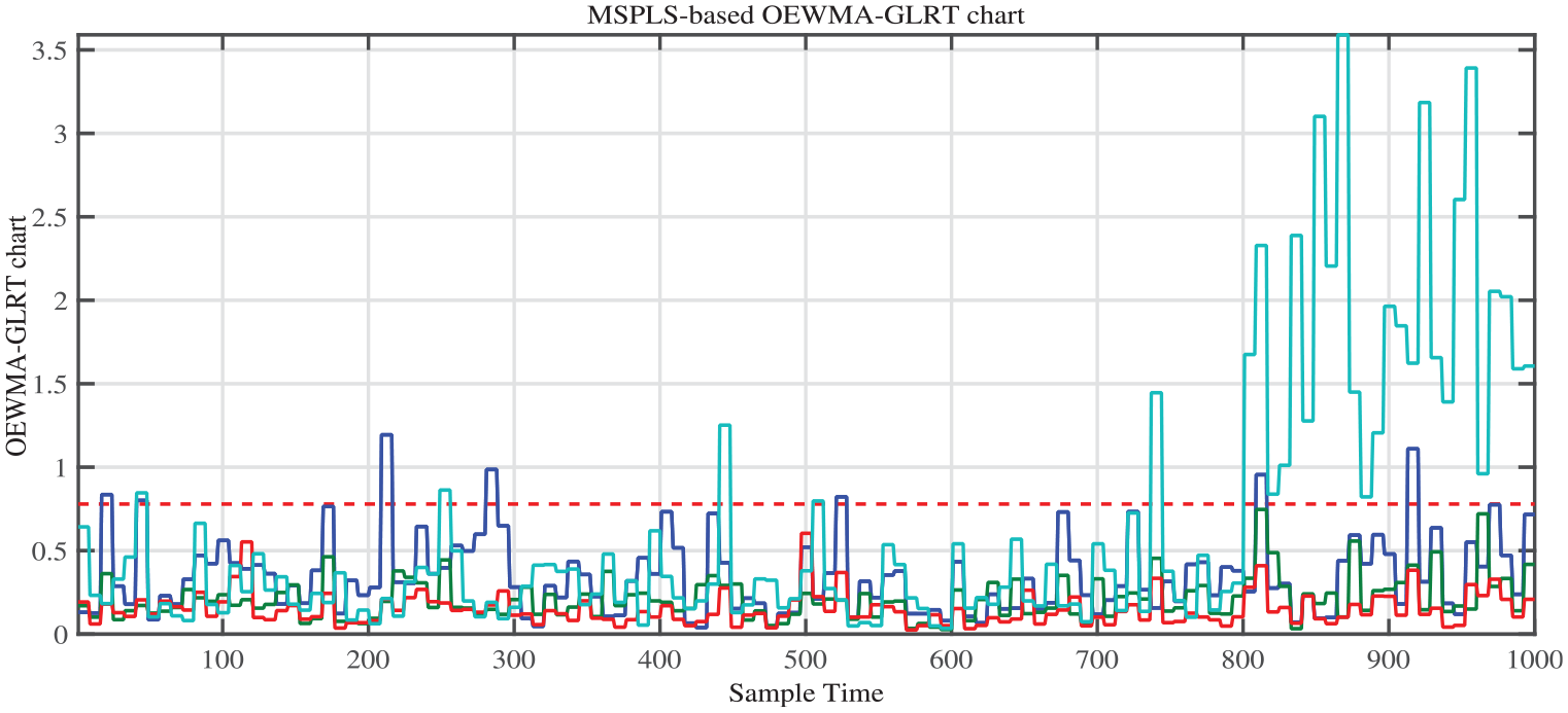
Results using MSPLS-based OEWMA-GLRT method.

Results using MSKPLS-based OEWMA-GLRT method.
MDR, FAR, and
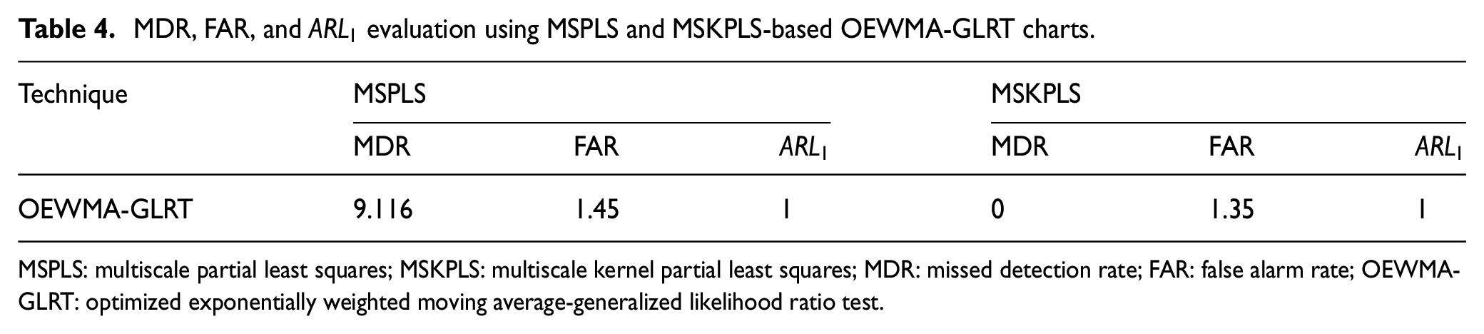
MSPLS: multiscale partial least squares; MSKPLS: multiscale kernel partial least squares; MDR: missed detection rate; FAR: false alarm rate; OEWMA-GLRT: optimized exponentially weighted moving average-generalized likelihood ratio test.
Conclusion
In this work, a MSKPLS-based OEWMA and GLRT is proposed for FD. The MSKPLS method is applied for modeling and OEWMA-GLRT chart is used for detection. The developed OEWMA-GLRT consists of computing an optimal statistic that merges current and previous information providing more importance to the most recent data. It chooses the optimal tuning parameters that minimize the MDR, the FAR, and the out-of-control average run length
Footnotes
Handling Editor: James Baldwin
Declaration of conflicting interests
The author(s) declared no potential conflicts of interest with respect to the research, authorship, and/or publication of this article.
Funding
The author(s) disclosed receipt of the following financial support for the research, authorship, and/or publication of this article: This work was made possible by NPRP grant NPRP9-330-2-140 from the Qatar National Research Fund (a member of Qatar Foundation). The statements made herein are solely the responsibility of the authors.