Designing a dynamic protocol for real-time Industrial Internet of Things-based applications by efficient management of system resources

Abstract

Wireless sensor networks have gained the attention of researchers from various fields due to increased applicability. This has thus led to rapid development in the field. However, these networks still suffer from various challenges and limitations. These range from computation and processing power and available energy to mention but a few. These problems are even much more pronounced in some areas of the field such as real-time Internet of Things-based applications. In this study, a dynamic protocol that efficiently utilizes the available resources is proposed. The protocol employs five developed algorithms that aid the data transmission, neighbor, and optimal path finding processes. The protocol can be utilized in, but not limited to, real-time large-data streaming applications. The protocol is implemented on sensor nodes that are custom made by our research team. In this article, a structure that enables the sensor devices to communicate with each other over their local network or Internet as required in order to preserve the available resources is defined. Both theoretical and experimental result analyses of the entire protocol in general and individual algorithms are also performed.

Introduction

Wireless sensor networks (WSNs) were introduced in the mid-20th century. They are distinguished from other network types by the large number of mini-sized sensor nodes and are characterized by relatively fewer sink/base station (BS) nodes. Each sensor node is equipped with sensing, processing, transceiver, and power supply units—normally in the form of a battery. Today, this field of study is rapidly spreading and various applications are emerging, for example, healthcare, ¹ agriculture, ² Internet of Things (IoT), ³ and fog computing. ⁴ The used sensor nodes possess limited power supply and overall processing capabilities. ⁵ Thus, the subunits and related protocols are required to efficiently use the available energy lest the lifetime of the node, in particular, and the WSN, in general, be shortened. Hence, most researchers have recently focused on solving these problems, especially the energy problem. Despite energy saving posing a trade-off with other design factors, namely, reliability and system overhead, it is required that a balance should be maintained between all the design factors. ⁶ It is necessary to pay attention to the needs of the application area to be designed while focusing on this goal. In these networks, one of the key application areas is real-time data streaming systems. Real-time image and video processing in wireless multimedia sensor network (WMSN) applications can be referred to as some of the many examples in this area. In particular, the suitable design model is an important requirement in real-time large data transmission.

It is of paramount importance that the designer should possess sufficient information about the design factors, communication architecture, and the stack protocol of WSNs while designing appropriate protocols. The design factors of a WSN are often standard in the implementation of a protocol. ⁷ However, it may vary depending on the goals of the implementation. For example, since the main goal of this study is to obtain efficient big data in real-time applications, greater priority will be given to data delivery, delay, and energy efficiency than to the other design factors. Therefore, a dynamic protocol that ensures optimal energy conservation and usage of the processing unit is proposed in this study. In addition, data aggregation plays an important role.

The sensor devices can collect large amounts of data from their environment easily and provide large data formation in the network. This data volume can lead to the creation of big data. This means that the collected data should be cleaned and compressed. These goals can be realized in data aggregation methods. The data aggregation is one of the key challenges in big data WSNs. It allows combining data from different sources to eliminate the redundancy and consequently reduce the consumption of resources available in the network. In the proposed protocol, the BS nodes, like fog nodes, perform the data aggregation processes. As the day goes by, the prevalence of these network structures is increasing, and in these structures, big data generation has become inevitable. Therefore, the importance of IoT-based applications is increasing exponentially. Effective management of the resources such as energy and processing power is thus of paramount importance.

Energy efficiency is debatable in all layers of the protocol stack. For example, in the study by Niewiadomska et al., ⁸ collision, packet overhead, latency, overhearing, and idle listening are discussed, and it focuses on their management to obtain energy efficiency. Collisions should be controlled because they cause unnecessary transmission costs at the source and destination nodes. Collisions can be managed in the design phase by using time-division multiple access (TDMA) and/or similar avoidance protocols. The other important issue in these networks is the limited power of the processor. Limitation in the processing unit can be solved by using various methods, for example, efficiently using packet sizes and developing efficient algorithms. ⁹ This issue has been addressed in very few research case studies most of which only dealt with it using methods such as data compression and data cleansing. On the contrary, decentralization of the architecture is one of the promising ways to achieve energy saving, which refers to distributing computation tasks to sensor nodes rather than executing them in a centralized architecture. In fact, the architecture of IoT-based applications, which are able to generate large amounts of data, is often of the centralized model. This type of architecture leads to excessive energy consumption in the network. ¹⁰

In IoT, devices are always connected to the Internet. This does not necessarily have to be the case. Some devices can be disconnected from the Internet and only connected when the need arises. Not every node can use many resources such as power and network bandwidth efficiently if it tries stream large data to the server or other nodes over the Internet. In addition, security and bandwidth problems are increasing in devices that are constantly connected to the Internet. Therefore, IoT devices do not always have to provide data streaming over the Internet. Devices on the same WSN can more efficiently save resources by streaming data over the network without necessarily connecting to the Internet. On the contrary, the protocol should be able to let the devices connect to the Internet when required. For example, if the BS wishes to broadcast a packet to a network whose area is much larger than its transmission range, instead of using the hop wise method, it may be faster and more efficient to broadcast the packet over the Internet. The management of these needs should be provided by the used protocol. For example, WMSN and wireless body sensor network (WBSN) applications can be implemented more efficiently with the proposed structure. These networks are already capable of generating big volumes of data. Data volume reduction is a particularly very important requirement when many packets of data are being sent over the network. There are rare scenarios in the literature where large volumes of data are transmitted. In the new world of information, data are allowed to grow with the intention of obtaining valuable information from it by the designers. Data analysis plays a very important role in obtaining the valuable information from such generated huge volume data in various applications, hence, the daily increase in its importance.

In real-time and big data-oriented applications, such as IoT-based applications, the devices (things) are able to communicate with each other from both the Internet and the local network. In this article, we introduce IoT and Network of Things (NoT) concepts that can work together. Each node is able to dynamically switch between the relative modules according to system requirements. Therefore, we design a network and propose a dynamic protocol in which nodes can communicate with each other both over the network and over the Internet. The proposed protocol benefits from the advantages of each of the aforementioned modes. The proposed protocol can be used in different scenarios: both in structures that have Internet access and those that do not according to the specifications and requirements of the system. This study mainly focuses on IoT- and NoT-based real-time applications.

A smart system based on WSNs consists of two parts in general: network and user (server) sides, as shown in Figure 1.All events are detected by sensor nodes and are converted to digital data by the analog to digital converter (ADC) subunit. Then, they try passing their data to the BS via the intermediate nodes using a multi-hop system. Finally, the BS/sink node sends all the received data to the server via Internet as one block or in parts. Therefore, data format and volume are sensitive issues that need attention in system design. The sensor nodes should use optimized data formats in transmission; also, they need to clean and compress the data before transmission. This way, the protocol can efficiently use both the processing and power units. In this article, a custom packet structure to obtain efficient results is defined.

Figure 1.

The working model of WSNs. ⁶

Data report techniques are usually four types in WSNs: event-based, query-based, time-driven, and hybrid types. In any case, the proposed protocols should have a solution to energy saving and data reduction. In practice, hybrid models appear more often on the front pages. This is because they can flexibly switch between techniques depending on the requirements.

In large-data application areas, the event-based technique is generally used but hybrid can also be used. Event-based systems are well known for generating large streams of data, which require fast processing of the incoming data. However, with the fast development of mobile, pervasive, and sensor-based technologies, data streams have become common in many applications. Such data streams show new and different features when compared to traditional data streams. On one hand, such data streams are unlimited in time (i.e. there is a continuous data stream generation), and on the other hand, the data size can be huge. Thus, many Internet-based applications produce large amounts of data, which are known as large data streams. Such applications comprise IoT-based monitoring systems and data analytics from monitoring online ad hoc systems.

As mentioned earlier, energy efficiency is one of the important factors in system design. Energy consumption in the transceiver unit is more than that of the other units (processing and sensing). A sensor node can be in two modes after deploying on the operation environment. First is the wake (active) state, and the other is the sleep state. Sleep and wake up modes and their effects on power consumption of each node are shown in Figure 2.

Figure 2.

A view of states node and power consumption. ¹¹

Therefore, energy conservation methods play an important role in WSNs. These methods are presented in three categories as shown in Figure 3. Several methods for energy saving in the network exist, such as data aggregation, switching sensor modes, keeping the network in connective state, learning methods for finding paths, and media access control (MAC) protocols (e.g. when to use collision management in the network) as shown in Figure 3.

Figure 3.

Energy efficiency schemes in the WSN.^6,12

Therefore, when a routing protocol is being developed, energy conservation can be achieved using one or more methods depending on the system’s requirements. The routing protocols in these networks may be concerned with various parameters such as Quality of Service (QoS), high-speed data transmission, reliable data transmission, reducing packet losses and packet delays, increasing network lifetime, and optimizing overhead of network by considering resource limitation. Many current algorithms and routing protocols can be classified into one of the flat, hierarchical, and location-based groups. ⁶ Hierarchical routing protocols have better performance than the other routing methods as far as energy efficiency is concerned. The fact that hierarchy methods are good at energy efficiency does not mean that the methods in the other group are not suitable. Network protocols are dependent on application types and their requirements.^5,6,12 In hierarchically based protocols, networks are divided into clusters. Each of the clusters has a cluster head (CH) node as the coordinator.^13,14 Therefore, the overall data volume of the network and load on the nodes is decreased.

Today’s observation streams of large numbers of geographically distributed sensors in the WSNs arrive continuously at powerful servers, and users are interested in analyzing the sensor data streams in real time. ¹⁵ In the high-volume data stream in the traditional networks, there exist many techniques for reducing the data volume such as sampling, histograms, sliding windows, and sketch techniques. These can be implemented on the WSNs but will not be efficient exactly due to limitation in the sensor resources. Therefore, the use or proposal of techniques is related to the type of applications and their requirements. For example, in the monitoring-based applications, the nodes only process their data and in the transaction-based applications, the nodes can interfere on the data. The data reduction importance is rising when our data lengths are large and we have big stream. The most common sensor stream solutions consider the network as a distributed database. In this case, the network abstraction is based on a data stream management system (DSMS). These applications are concerned with how can be answered.^15–18 Some proposals use the amount of resources available at a DSMS and apply it to extract management information from the WSN, such as energy and node location.^19,20 However, current DSMSs are not suitable for WSNs, since sensor nodes have too few resources.

In the literature, studies focusing on data streaming techniques over WSNs can be found. In some cases, the application performs an adaptive sampling of the data sensing.^21–24 In other cases, the solutions are based on data reduction or aggregation, often based on correlated information about the data sensing.^25–28 Diallo et al. ²⁹ suggested an adaptive method for WSNs to reduce the network traffic retaining the data quality and its representativeness. If a node sends all its measurements, it will spend much energy, and part of the data can probably be delayed or lost. Diallo et al. ²⁹ believed that, to avoid this, part of the data is just not processed. However, intervention of data in large data stream scenarios is not mentioned. The large data stream is even further magnified at two parts of system (both inside the network and at the server side).

We are mainly concerned with the data management issue inside the network at every sensor node in our proposed protocol. Data management is realized using different approaches such as defining suitable data frame structures and cross-checking for differences in the sent and received packets. In addition, we focus on data reduction using data-driven methods such as data aggregation based on our semi-dynamic data frame templates. Last but not the least, energy efficiency is realized based on duty cycle and data-driven methods for high volume data streams in the network. All the aforementioned will be applied to and implemented in our proposed dynamic protocol wherever necessary.

In this article, we are focusing on real-time IoT-based applications by efficient management of system resources such as power and bandwidth. In the real-time-based large data size applications, the network resource management is very important, so the selection of appropriate sensor nodes and management of their nodes and route election are critical issues in these applications. For this reason, we need to propose an efficient protocol with suitable packet frame. We define a custom structure model for network deploying and realizing network connectivity. The proper data pattern definition and network configuration play a major role in the efficient use of resources. After these operations, an efficient routing protocol will need to be defined. For this purpose, the nodes need to recognize a method that optimizes their neighbors. In addition, the pathfinder algorithm will be proposed. Also, three different data transmission algorithms will be proposed for different scenarios and application fields. This diversity will ensure that the protocol in this study can be used for wide coverage in IIoT systems with different real-time data. In fact, in this study, only one protocol is not recommended; perhaps, a method is suggested that provides diversity that can meet the needs of the field of related application. Thanks to this, the implementing companies and scientists can use the proposed approaches in this study in their field and laboratory studies and they will be able to contribute to this field with the improvements they can get.

In this section, an introduction to big data WSNs and real-time IoT-based applications are given, and the related works are explored. The rest of this article is organized as follows: in section “Research method,” the proposed dynamic protocol is introduced. In section “Evaluation of the proposed protocol,” evaluation and theoretical analysis of the protocol are presented. In section “Testbed experiment results,” the obtained experimental results are provided. Finally, the conclusion and future works are discussed in section “Conclusion and future works.”

Research method

In this section, a dynamic protocol is proposed for usage in large-data real-time applications. It is a general multi-purpose fundamental protocol that can be used in a wide range of systems and structures for various applications such as WMSN- and IoT-based applications.

We design a structure in which sensor devices are enabled to communicate with one another over their local networks or Internet as and when required. Given a sensor stream, we want to meet WSN requirements by reducing data traffic (using techniques based on data stream) and assuring a minimum data length in order to decrease energy consumption and delay rates. To achieve this feat, we need to pre-define a few terms as will be applied to the proposed protocol. Some of these are as follows: the network topology over which the protocol is applied and data stream generation and processing methods. In our network topology, we have a flat network structure composed of sensor nodes with a single BS to receive and process data from the nodes. For stream data processing, each node locally processes its own data stream first and then sends the results toward its neighboring nodes, that is, data processing is not only done by the BS. Data streams are generated continuously at regular intervals (network rounds) of time and are followed as a normal distribution to represent their values. It is necessary to pay attention to the characteristics of the large data streams such as volume, velocity/rate, variety, veracity, and value. ³⁰

The expectations from the system are acceptable network lifetime and delay and data reliability rate. Given these goals, load balancing in the network should be put under consideration because, as mentioned earlier, some parameters have trade-offs with each other. In this section, first, we will explain our designed sensor node structure and then the proposed protocol.

Hardware of our sensor nodes

In this section, we introduce and, in detail, explain our newly designed sensor node kit. Figure 4 shows one of the custom-made sensor nodes that Robotistan-Sixfab Company commissioned it according to the request and idea definition of IZU-WSN laboratory team. The original designer of this product and the rightful owner is Robotistan-Sixfab Co. ³² The entire kit is known and will henceforth be referred to as the KIANI-WSN kit.

Figure 4.

Our jointly produced sensor and gateway nodes. ³¹

These nodes consist of four main units and these are the sensing, processing, transmitter, and power units. The transmitter unit is equipped with a Wi-Fi card and a specific module produced by Texas University. ³³ Our nodes are in two production categories. One of them is of sensor nodes that are equipped with the CC1101 transmitter chip and other is of nodes that are equipped with both the CC1101 and the CC1190 chips. The latter serve as our gateway (BS) nodes. These chips are Texas University products, so we used them as transmitters in our sensor node design in addition to the Wi-Fi module.

CC1101 is a low-cost sub-1 GHz transceiver that is usable in very low-power wireless-based applications. It supports 315, 433, 868, and 915 MHz bands but we used 868 MHz band because this bandwidth is available in the European regions. The radio frequency (RF) transceiver is integrated with a highly configurable baseband modem. The modem supports various modulation formats and has a configurable data rate up to 600 KBps. ³³ The CC1101 also supports the packet handling, data buffering, burst transmissions, clear channel assessment, link quality indication, and wake-on-radio. The main operating parameters and the 64-byte transmit/receive first-in-first-outs (FIFOs) of CC1101 can be controlled via a serial peripheral interface (SPI). It supports node communication with 100 m distance in line of sight (LoS). The CC1190 850–950 MHz range extender ³⁴ can be used with CC1101 in long-range applications for improved sensitivity and higher output power. The coverage range of our gateway nodes can be up to several kilometers in LoS.

The sensing unit consists of ADC section and 12 pins for sensors, so we can add maximum 12 sensors to sensing different environment based on requirements of the applications. Other unit is the processing unit that has been used as a microprocessor of Atmel series in it. This microprocessor is working in 16 kHz, and it can process 16 million cycles per second approximately. The third unit is the transceiver unit, so it works in the RF module, and it is based on Texas University products as described earlier. Last unit is the power unit that indicates the power source of the sensor node.

Proposed protocol

The proposed dynamic protocol in this article comprises two phases: network configuration and routing. In this section, five algorithms are proposed to serve different purposes. One of them is neighbor finding, the other is pathfinding, and three algorithms to aid in data transmission for different scenarios. Furthermore, the evaluation of all proposed algorithms is discussed in detail in the next section.

The network configuration phase consists of three parts: custom data frame definition, building efficient network structure, and introducing a neighbor-finding algorithm, whereas the routing phase consists of two major parts: pathfinding and data transmission. All methods are described in this section.

Energy conservation in our protocol is based on sleep/wake up, data aggregation, and node density regulation methods. To manage sleep/wake up, on-demand, synchronous, and asynchronous techniques are used as shown in Figure 3. The TDMA method was used for channel management, while the code-division multiple access (CDMA) method was used for collision control. We also used the carrier-sense multiple access (CSMA)-MAC protocol so that our protocol could work well in the mobile target-based applications. Congestion control is also achieved by buffer size control and time stamp application methods.

Custom data frame

The first step of the configuration phase is custom data frame definition. But for the hard-coded requirements of the node hardware such as the sync word (synchronization word), our custom-made nodes were designed in such a way that enables the researcher to design and reconfigure the data frame structure as they see fit. Fields such as data length can be reconfigured.

A general data frame structure to be used in various applications is shown in Figure 5. In some applications, some fields may not be required. Those fields of the data frame can be left blank. As a part of the future works, the data frame structure will be dynamically generated depending on required fields of the application in question. This structure is predicted to be used in a system with learning capabilities. In this article, our data frames are a total of 69 bytes and the data field size can be up to 52 bytes, as shown in Figure 5.

Figure 5.

Our modified data frame.

These fields are defined according to the data frames used in WSNs and wireless communications, ³³ as well as the possible needs of application areas. The first field of the proposed custom data frame is the preamble pattern. It is an alternating sequence of ones and zeros (10101010…). The minimum length of the preamble is programmable. When enabling TX, the modulator will start transmitting the preamble. After the programmed number of preamble bytes has been transmitted, the modulator will send the sync word and then data from the TX FIFO queue if data are available. If the TX FIFO queue is empty, the modulator will continue to send preamble bytes until the first byte is written to the TX FIFO queue. The modulator will then send the sync word and then the data bytes. Sync word is a two-byte value that provides byte synchronization of the incoming packet. Cyclic redundancy check (CRC) is a simple 16-bit CRC field that automatically calculated and appended by the CC11XX IC, based on the contents of the CC11XX data payload. Network ID means maybe we have more than one network and maybe packets interrupted. Cluster ID indicates our cluster number/layer number when the network structure is cluster based. Type and subtype fields determine the type of frames. Our frames can be status, query, and data. Subtypes can indicate different information such as energy reminder, channel status, buffer size status, neighbor finder, distances, acknowledgement (ACK), request to send (RTS), clear to send (CTS), authentications, and null frames. MP (more packet) means that more packets will follow. Power status indicates that the sender is going into power-save mode in sleep or wake up mode. Priority indicates the rate of packet priority. It can be used for sending emergency data. If the field value is high, it shows high priority level.

Network structure based on the virtual layer

As mentioned earlier, the network is assumed to be a flat structure that uses the new method for creating virtual layers similar to hierarchy. In this way, we combine the advantages of both flat-based methods and hierarchical methods. In this model, each node processes and reduces the received data packets before forwarding them to its neighbors. In this phase, first step is node deployment. Distribution of nodes in the environment can be done randomly or manually. Then, each sensor node should know its neighbor’s information using RF coverage. The number of shapes and sizes of virtual layers can be variable. This structure increases the applicability of the proposed method to various fields.

The proposed virtual layer structure for our network yields reduced energy consumption. We define a variable C, connectivity degree, in each layer. After generating virtual layers, all nodes in each layer are modeled as a random graph. Each node waits for a random amount of time, t_v, uniformly distributed in the range (0, T). After t_v time units, a node operates actively for T time units. At first, it broadcasts a HELLO message to announce its activation to its neighbor nodes in the same layer. The node can then go to sleep after T time units until the next period—as soon as it receives C messages from its neighbors. C is the connectivity degree, and T is the duty cycling period. In each layer, the value of C may vary according to the network size and the volume of data sent. The selected nodes for data transmission cannot affect the value of C until their tasks are finished. Hence, the protocol needs to adjust the C value regardless of these nodes. In the example presented in Figure 6, the C value is 8. In this case, eight of the nodes that are in each other’s transmission range in each layer will be active, and the others will be put in sleep mode as shown in Figure 6. The value of C is chosen by the protocol in such a way that all the nodes in a given layer are covered.

Figure 6.

An example of communications and topology schema when C = 8. ⁶

The nodes that are in sleep mode activate their radios for a short time and send their packets to one of their neighboring active nodes if it is not yet their turn to be active and they have got packets to send. This scenario can arise say during the pathfinder process, or if the sleeping nodes’ buffers are not empty. This is shown in Figure 7.

Figure 7.

Packet routing in sleeping nodes.

Neighbor finder method

As mentioned earlier, the second step of network configuration is neighbor finding. It can be realized after the deployment process. In this section, we propose a method by which each node can find its neighbors. Each node can find its neighbors based on its RF coverage area. In this method, first, the BS broadcasts the HELLO packet with a variable called hop. The initial value of this variable is zero. We use the hop variable for creating virtual layers in this algorithm, so any nodes will know how many hops they must have to reach BS. Each node will compare the hop value of the received packet with own hop value. If the received hop value is less than its value, it saves the received value in its value and sets its layer number with this value. Then, it increases the value of the corresponding variable by one unit and broadcasts the HELLO packet to its neighbors. This process will continue until all nodes on the network receive this packet. A simple example of this structure is shown in Figure 8. The initial hop value of each node is infinite number. The set of (S, T, packet, counter) is for avoiding getting redundant packets. This technique is used in all methods of the proposed protocol. The fields of the HELLO packet is presented below, where mean of BC is the broadcasting type, 00 indicates the status (management) type, and 0001 indicates the neighbor finder subtype

$$\mathrm{HELLO}(\mathrm{S},\mathrm{BC},00,0001,\mathrm{cost}\mathrm{-}\mathrm{BS},\mathrm{packe}{\mathrm{t}}_{\mathrm{id}},\mathrm{counter},\mathrm{hop})$$

The pseudocode of the neighbor finder algorithm is presented in Figure 9.

Figure 8.

The scenario of the neighbor and layer finder method by the virtual layer method. ⁶

Figure 9.

Pseudo code for neighbor, cost finding, and creating routing table.

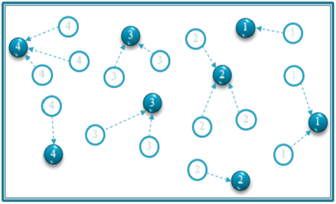
As a result of this method, any node will know its layer, neighbors, its layer neighbors, and its cost between BS and its neighbors. According to this information, each node can set its routing table. A simple example is presented in Figure 10 of the routing tables’ creation. The cost between two neighbor nodes is based on TX-power and received signal strength indicator (RSSI) values. In addition, the costs between any nodes to BS are calculated directly or indirectly with their remaining energy rates. Another special aspect of this method is that the costs between the nodes in the same layer are also calculated. As a result, all nodes of networks will have created their routing tables with three columns (cost-BS, cost-neighbors, and layer-number), so their values are calculated as shown in Figure 10 as a sample work. In this figure, the blue arrows are accepted packets because the hop value of receiver node (hop_id) is more than the hop value. As mentioned earlier, the initial value of hop is infinite in all network nodes and zero in BS. The red arrows show discarded packets when the hop_id is less than hop value and yellow arrows indicate the relations of the nodes in the same layer that hop_id is equal with the hop value.

Figure 10.

Creation of routing tables of each node in the neighbor finder algorithm.

After finishing the deploying network and creating routing tables, the protocol should find the possible optimum routes between network nodes. For this, the pathfinder method is recommended. In this method, real-time- and large-data-based applications are considered.

Pathfinder method

In this section, a pathfinder algorithm is proposed to find the possible routes and best path between the sender and target (destination) nodes. It is first step of the routing phase. It is started when a datum is available for sending. The pseudocode of the proposed algorithm is presented in Figure 11. It is running in opposite directions. In first, direction is from source node (S) to target node (T), when a source node wants to send its data as real time to T. In second, the direction will be from T to S node when the algorithm found the T node and wanted answer to the S node. Packets sent from S to T are called RReq, and the packets sent in the opposite direction are called RRep. The formats of RReq and RRep are introduced in our custom data frame that the frame generally explained in the before section

$$\begin{array}{l}\mathrm{RReq}\left({\mathrm{S},\mathrm{T},01,1000,\mathrm{packet}}_{\mathrm{id}},\mathrm{counter},\mathrm{hop},\mathrm{data}-\mathrm{length}\right)\\ \mathrm{RRep}\left({\mathrm{T},\mathrm{S},01,1001,\mathrm{Cost}-\mathrm{T},\mathrm{from},\mathrm{packet}}_{\mathrm{id}},\mathrm{counter},\mathrm{hop},\mathrm{age},\mathrm{data}-\mathrm{length}\right)\end{array}$$

where “01” specifies query type, “1000” subtype means RTS, and “1001” is CTS. The “Cost-T” presents cost of each sender node to T; “from” is address of sender node. The age in milliseconds for which nodes receiving the RRep consider the route to be valid. “Data-length” is created by the S node in the first step. Any receiver node calculates its cost values based on this length, so each node can check whether there is enough resource to send these data.

Figure 11.

Pseudo code of the pathfinder algorithm.

The mechanism of this algorithm is described below. Initially, the source node (S) broadcasts the RReq packet to its neighbors. The receiver nodes (node_id) check their address with T address. If the T node is one of the receivers, T and S are adjacent to each other. In this case, the proposed method will find the routes between them in very short time. If none of the receivers are T, each of them check the packet that whether they have taken it before. The checking operation is done by S, T, packet_id, and counter parameters. The nodes who have not received it before, broadcast the RReq to their neighbors. This process will continue until the T node is found.

The second stage of the algorithm will start with the presence of T node. As soon as the corresponding node is found, the packet traffic will be realized by broadcasting RRep to its neighbors. In this process, any node updates its cost to T and sends the corresponding packet to its adjacent. Each node checks received hop value with the self-hop value for accepting or denying the packets. If the received packet hop value is less than the self-hop value, it will get these packets from all possible neighbor nodes and update the cost value. It uses a minimum value of cost in the sending phase. The most specific part of this algorithm is the behavior of the nodes in the same layer. Each receiver node searches layer number values in its routing table. Any row that has the same value as the receiver layer number specifies that the nodes are in the same layer. If the receiver node has such neighbors, it compares its cost value with the layer-neighbor cost value and chooses the smallest value (6.3. part of Figure 11). The broadcasting in the second stage may start after these processes. Thus, nodes always get the packets that have the lowest cost.

The proposed algorithm does not just focus on the limited parameters such as distance and node battery rate in the cost updating process. It concerns to channel and buffer status besides these. In addition, it gives weights to each parameter. It pays attention to appropriate values according to the importance of amounts and effect coefficient of resources on the network.

The example of the working model of this algorithm is shown in Figure 12. In this example, T starts the broadcasting of RRep upon receipt of the request packet. It adds its cost and sends to its neighbors. The receiver nodes update their cost to T and store it and sender_id in their local memory, then, send the RRep to their neighbors again. When a node receives more than one valid packet from its neighbors, it stores and sends the minimum cost value to T (i.e. S node behavior in Figure 12). As mentioned in pathfinder pseudo code, in the packet transmission between same layer nodes, these nodes can send RRep to their neighbors after finding the minimum cost to T.

Figure 12.

An example of the proposed path-finding algorithm.

In the real-time large-data stream scenarios, using the allocated channel has better performance in data delivery rate. In the cost calculation steps, each node considers the size of the data (that will be sent from S to T) and its resources. This feature of the proposed algorithm allows the nodes to send the accurate information to each other. In addition, any node that has been collaborated in the data transmission as the minimal best route should update its values of resources because it spends its resource in this transmission process. Thus, the pathfinder algorithm always can find best routes because the algorithm knows this information of the resource status of nodes. Therefore, the reliability rate of the proposed protocol will be high in the real-time large-data stream-based applications.

As a result of the pathfinder algorithm, each source node finds best route to reach to its T node. Reserving this path for the entire data transfer depends on the data transmission algorithm used. For this reason, three different data transmission algorithms are proposed. As mentioned earlier, the second phase of the proposed protocol is data transmission. The designer decides from the beginning whether to use the algorithm according to the field of application in which the protocol is to be used, or he or she may provide different algorithms for different processing conditions by defining certain conditions.

Data transmission method

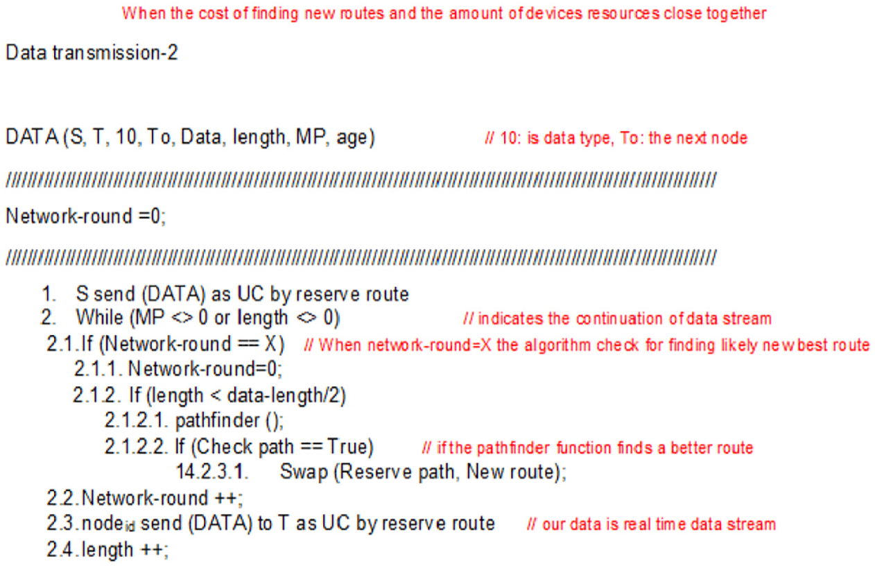
In this section, three algorithms for data transmission that are usable in different scenarios depending on the hardware and application requirements are proposed. They are presented as pseudocode in Figures 13–15, respectively. It is the last part of the routing phase. The first algorithm, as shown in Figure 13, uses the best route for data transmission based on the result of pathfinder function. However, it will call the pathfinder function at certain running rounds of network, which we named this parameter NR. It is a widespread method for evaluating network-operating times within certain rounds.^6,11,12 It calls the corresponding function, when the network round value is equal to our certain value. Therefore, it spends more energy and processing clocks. However, the selected nodes can consume less energy if the pathfinder function can find other alternative best path. The nodes on the selected best path consume more energy than other nodes. Hence, it is likely to find a new best route.

Figure 13.

The pseudo code of the first data transmission algorithm.

Figure 14.

The pseudo code of the second data transmission algorithm.

Figure 15.

The pseudo code of the third data transmission algorithm.

The MP variable used in this algorithm indicates that more packets will follow. It means that there is a continuation of packets when the value is zero, and its value in the last packet of data is one. Length filed indicates the remaining transmitting data length from S to T. Every node on the best route (path) knows the total data length before staring data transmission. This information has been reported to any node by S node in the pathfinder phase. The nodes in the best route send data as unicast until the end of the data transmission process.

The first data transmission algorithm allows us to use other alternate routes in this process. In this algorithm, the data transfer rate does not only stay on the nodes in the optimal path but also gives a chance to other network nodes to collaborate in the data transmission process. In this case, the data transmission load of the network can be divided into a balance, if the pathfinder function finds new best routes. Because of its cost and more energy consumption in the processing and transceiver units, this algorithm is suitable for applications that the priority of data transmission time is less than the energy consumption rate. It is worth mentioning that finding new routes can decrease energy consumption on the nodes that were elected for current path. Indeed, this method effect may be temporarily on the path nodes and not on the whole network lifetime. It does not mean that there is no chance that it will affect the whole network life, and it depends on the application area, environment condition, network architecture, and topologies. Since the cost of nodes for the transmission of each data is calculated based on the volume of data, the whole transmission of data on the current best route is possible by elected nodes. Yet, these nodes will have less energy for the next data transmission processes, consequently, election chance of them will be decreased. The algorithm evaluation details are explained in the next section.

The second proposed algorithm is more focused on the balancing between packet delays/delivery and energy consumption. It does not transmit all packets of the data over a single route, and it gives a chance to other possible routes similar to the first algorithm. However, it pays attention to the amount of the remaining data packets before calling the pathfinder function. It calls the relevant function if the remaining data volume has its worth to energy consumption rate. Otherwise, it continues to data transmission on the current path. The details of the second algorithm are shown in Figure 14 as a pseudocode.

The third proposed algorithm uses the result of pathfinder function and transmits all packets of the data on the selected best route until the end of packets. It focuses on data transmission without delays only. It also has acceptable performance in energy consumption, when our evaluation is on one-to-one data transmission. However, we need to focus on all the data that should be transmitted on the network. The details of the third algorithm are shown in Figure 15 as a pseudocode. In this algorithm, the selected nodes in the first best path spend more energy than the other two algorithm nodes. However, these nodes are not prone to premature energy consumption, because the probabilities of being selected will be lower than the other nodes. There is only one certain issue that it is the pathfinder function cost. Of course, it may have no effect in the whole network.

Therefore, the performance of algorithms is related to the requirements of applications. For example, we can have different exceptions as the following example, which is also shown in Figure 16. The third algorithm does not have a good performance in delay parameter when Z node wants to send its data to destination node (T), so it has one possible route to reach to T only. Therefore, in this case, the first and second algorithms have better performance than the third algorithm. The third algorithm can also lead to starvation. It is necessary to select the most suitable algorithm/algorithms according to the needs of the system to be designed. The function of each of the three algorithms in this scenario is shown in Figure 16.

Figure 16.

An example of the possible exceptions in the data transmission.

In general, in this article, a protocol with five different algorithms is proposed. The proposed protocol does not select nodes with limited resources in the best route finding process because it checks different parameters of nodes such as their battery level, channel status, buffer status, and the size of the data. For this reason, the probability of failed or loss routes in the proposed protocol is low. However, the protocol calls the pathfinder algorithm to find an optimal route in the case of path failures due to various reasons ranging from node failure to environmental changes, among others. Therefore, the proposed protocol exhibits good performance when it comes to fault tolerance. On the contrary, the packet delivery rate is increased by using the check path function because this function checks other possible best routes between source and target nodes as alternative paths.

Evaluation of the proposed protocol

In this section, the proposed five algorithms are evaluated in various scenarios. The five algorithms are neighbor finder, pathfinder, and three versions of data transmission with diverse requirements. They can be used in various environments based on the application requirements. In order to calculate the cost of algorithms, we need to know the energy consumption rate of sensor nodes and overall cost of execution of each algorithm. All proposed algorithms are implemented on the produced our sensor nodes using the C++ programming language. Energy consumption evaluation of each node is based on send, receive, and sleep modes. Energy consumption rates in each mode are presented in Table 1.

Table 1.

Energy consumption rates in the Kiani node.^32,35

Initial battery of eachsensor node	1200 mAh
Current consumptionin receive mode	15.7 mA	Receive mode, 1.2 kBaud, reduced current, input at sensitivity limit
	14.7 mA	Receive mode, 1.2 kBaud, reduced current, input well above sensitivity limit
	15.6 mA	Receive mode, 38.4 kBaud, reduced current, input at sensitivity limit
	14.6 mA	Receive mode, 38.4 kBaud, reduced current, input well above sensitivity limit
	16.9 mA	Receive mode, 250 kBaud, reduced current, input at sensitivity limit
	15.6 mA	Receive mode, 250 kBaud, reduced current, input well above sensitivity limit
Current consumptionin send mode	30 mA	Transmit mode, +10 dBm output power
	16.8 mA	Transmit mode, 0 dBm output power
	13.1 mA	Transmit mode, –6 dBm output power

As mentioned earlier, our nodes were designed in two production categories: CC1101 and CC1190. They are configured using the SmartRF® Studio software. ³⁵ A screenshot of the SmartRF Studio user interface is shown in Figure 17. It is used in the initial setup of the nodes’ parameters such as the channel and buffer capacity, RF power in sensing and transmission, modulation method, and sync type.

Figure 17.

SmartRF^TM Studio ³⁵ User Interface.

Neighbor finder algorithm evaluation and complexity analysis

The complexity of our proposed algorithm in the neighbor and cost-BS finder phase in the processing unit is O(n). In addition, the energy consumption of the transceiver unit is a factor of n and m parameters as presented in equation (1), where n is number of network nodes and m is the total number of neighbors of all nodes in the network. In addition, E_s and E_R are the energy consumption rates in the send and receive modes, respectively. Details are presented in Table 4 in Appendix 1

$$\mathrm{Battery}{\mathrm{Cost}}_{\mathrm{neighborfinder}}=\left[{\mathrm{Cost}}_{\mathrm{send}}\right]+\left[{\mathrm{Cost}}_{\mathrm{Rec}.}\right]=\left[\mathrm{n}\times {\mathrm{E}}_s\right]+\left[2\mathrm{m}\times {\mathrm{E}}_R\right]$$

(1)

In our experiment, each node receives and sends one packet in 300 µs on average. Since the time difference for each process is negligibly small, always close to 300 µs, we fix this value to be 300 µs for convenience in the rest of this study. Indeed, that is, each node is doing two operations in total during this time. As mentioned earlier, our packet sizes are 69 bytes and the data size can be up to 52 bytes. Therefore, each node transmission near to 6666 packet numbers in per second that it equal with 460 KB packets and 345 KB data.

Also, based on the experiments performed using the presented algorithms and according to the datasheet of the employed nodes, presented in Table 1, each node consumes 0.016 and 0.019 mA to receive and send a packet, respectively. Therefore, assuming we have 100 nodes in our network and that the total number of edges is 200, we can transmit 460 KB packets per second expending a small amount of energy. A summary of the aforementioned scenario is presented in Table 2. This table shows some interesting information such as rates of data transmission and energy consumption per second.

Table 2.

Ability of each node in per second in normal condition.

Time	Packet size	Data size(maximum)	Packet number	Energy consumptionin receive mode	Energy consumption in transmit mode
1 s	460 KB	345 KB	6666	108 mA	122.4 mA

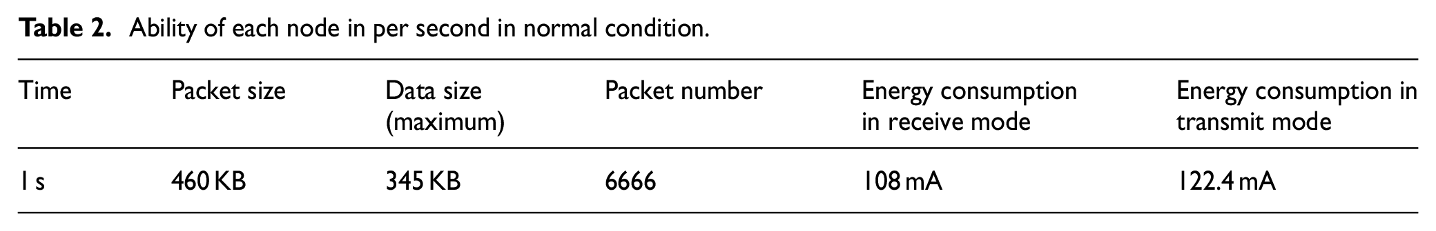
Therefore, the cost of the neighbor finder algorithm in the transceiver unit is 8.3 mA in the aforementioned example. This indicates that each node consumes 0.083 mA of its power unit. This value is acceptable in the whole network lifetime because each node can survive for 4,320,000 s (1200 mAh × 60 × 60). In fact, each node can send about 1.5 GB of data continuously under normal conditions, that is, assuming unexpected events such as node failure, and environmental changes do not occur. This amount increases with increase in network size if and only if network resources are used efficiently. If the aforementioned proposed algorithms are used in related applications, the value can be increased up to 2 GB—owing to the algorithms’ efficient usage of system resources, namely, power and processing unit. This value (2 GB) was empirically obtained from the performed tests. This amount indicates that the proposed method works well with devices and exhibits good performance in data transferring, so it is usable in the real-time large-data-based applications.

Pathfinder algorithm evaluation and complexity analysis

Evaluation of the pathfinder algorithm will be explained using a scenario tested out from one of the performed experiments. Assume that the number of sensor nodes in the network is 7 and that the number of all edges is 22 and the number of all neighborhoods that are in same layer is 6, as shown in Figure 18. In this example, the set A-B, B-A, B-C, C-B, E-D, and D-E all contain neighbor nodes in the same layers.

Figure 18.

An example of the network in the pathfinder phase.

The computational cost of this function is O(n)² in the worst case. This occurs when the number of records of the routing table of the receiver node is equal to that of the total nodes in the network. The cost of the algorithm under normal conditions is O(nd), so the d indicates the number of neighbors of each node. Energy consumption in the whole network is calculated using the following equation

$$\begin{array}{c}\multicolumn{1}{c}{\mathrm{Battery}\mathrm{Cos}{\mathrm{t}}_{\mathrm{pathfinder}}={[\mathrm{Cos}{\mathrm{t}}_{\mathrm{send}}+\mathrm{Cos}{\mathrm{t}}_{\mathrm{Rec}}]}_1}\\ \multicolumn{1}{c}{+{[\mathrm{Cos}{\mathrm{t}}_{\mathrm{send}}+\mathrm{Cos}{\mathrm{t}}_{\mathrm{Rec}}]}_2}\\ \multicolumn{1}{c}{=[(\mathrm{n}-1)\times {\mathrm{E}}_{\mathrm{S}}+2\mathrm{m}\times {\mathrm{E}}_{\mathrm{R}}]}\\ \multicolumn{1}{c}{+[((\mathrm{n}-1)+\mathrm{r})\times {\mathrm{E}}_{\mathrm{S}}+2\mathrm{m}\times {\mathrm{E}}_{\mathrm{R}}]}\end{array}$$

(2)

where n is the number of network nodes and m is the total number of neighbors of all nodes in the network. In addition, r indicates the total number of neighboring nodes in the same layer. Cost₁ indicates costs of the network when path direction is from S to T, and cost₂ is for the reverse direction. In the example presented in Figure 18, the energy consumption in the whole network is 1.046 mA as obtained using equation (2).

Data transmission algorithm evaluation and complexity analysis

Now, let us assume we have data of size 1 MB that should be sent from S to T in real time. As explained in section “Custom data frame,” our data frames are 69 bytes and can contain data of up to 52 bytes each. Therefore, 1 MB data can be sent using 19,230 packets, but we should send 25,517 packets. Required time to transmit each packet in the designed network was 150 µs on average (as mentioned in Table 2). Therefore, the whole data will be sent in approximately 3.83 s. The number of packets to be sent and the required times are calculated according to equations (3) and (4), respectively

$$\mathrm{c}=\frac{\frac{\mathrm{L}}{52\mathrm{B}}\times 69\mathrm{B}}{52\mathrm{B}}$$

(3)

$$\mathrm{required}\mathrm{times}=\mathrm{c}\times \mathrm{t}$$

(4)

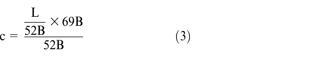
where L is the length of data that is to be sent and c is the corresponding number of packets. In addition, t is the required time to transmit/receive one packet. The value of t in the performed experiments was 150 µs on average.

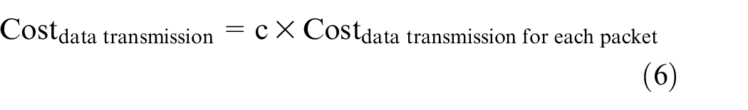
Energy consumption during data transmission depends on data length and number of nodes in the determined routes. The cost of data transmission is calculated using equation (6), derived from equation (5). Equation (5) calculates the cost of data transmission for each packet in the network, where y is the number of nodes that are selected during the best route finding process

$$\mathrm{Cos}{\mathrm{t}}_{\mathrm{data}\mathrm{transmission}-\mathrm{P}}=[(\mathrm{y}-1)\times {\mathrm{E}}_{\mathrm{S}}+(\mathrm{y}-1)\times {\mathrm{E}}_{\mathrm{R}}]$$

(5)

$$\mathrm{Cos}{\mathrm{t}}_{\mathrm{data}\mathrm{transmission}}=\mathrm{c}\times \mathrm{Cos}{\mathrm{t}}_{\mathrm{data}\mathrm{transmission}\mathrm{for}\mathrm{each}\mathrm{packet}}$$

(6)

First data transmission algorithm

Besides the overall costs, the complexity of each proposed algorithm in data transmission should be assessed. The general complexity of the first data transmission algorithm (DT₁) is O(cnd). It calls the pathfinder function during data transfer after every predetermined number of rounds. NR is the number of rounds, and NR_t is every round’s duration. For example, if NR_t per round is 300 ms, NR is incremented by one unit every 300 ms. If we suppose that the pathfinder function is called in each of four rounds, the cost of the DT₁ algorithm will be 2682.423 A. The computational cost of this algorithm is negligible for our processor because it supports 16 million clocks per second. However, it can be an important parameter in power consumption. The overall cost of DT₁ calculated as shown in equation (8), where, in our example, NR is 4, NR_t is 300 ms, and c is 25,517. These values can be set based on the designer’s requirements and goals. In our example, PF_count was considered to be 3

$${\mathrm{PF}}_{\mathrm{count}}=\mathrm{pathfinder}\mathrm{call}\mathrm{counts}=\frac{\mathrm{c}}{\mathrm{NR}\times \frac{\mathrm{N}{\mathrm{R}}_{\mathrm{t}}}{\mathrm{t}}}$$

(7)

$${\mathrm{Cost}}_{{\mathrm{DT}}_1}{=\mathrm{Cost}}_{\mathrm{data}\mathrm{transmission}}+\left({\mathrm{PF}}_{\mathrm{count}}{\times \mathrm{BatteryCost}}_{\mathrm{pathfinder}}\right)$$

(8)

Second data transmission algorithm

The cost of the second data transmission algorithm (DT₂) will be 2681.046 mA in this example, because it checks the remaining data size before calling the pathfinder function. Here, it calls the function once time. The algorithm will try to find new best routes like the DT₁. However, it pays attention to the amount of remaining data packets before calling the pathfinder function. DT₂ is more focused on the balancing between delays and energy consumption

$$\{\begin{array}{c}\mathrm{PF}=\mathrm{PF}+1\mathrm{if}\mathrm{NR}\times \frac{{\mathrm{NR}}_{\mathrm{t}}}{\mathrm{t}}<\frac{\mathrm{c}}{2}\\ \mathrm{PF}=0\mathrm{otherwise}\end{array}$$

(9)

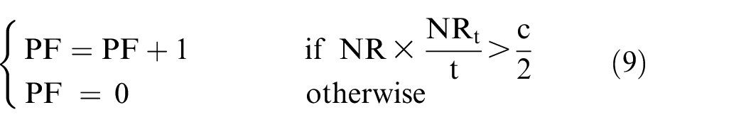
where initial value of PF is zero

$${\mathrm{Cost}}_{{\mathrm{DT}}_2}{=\mathrm{Cost}}_{\mathrm{data}\mathrm{transmission}}+\left({\mathrm{PF}\times \mathrm{Battery}\mathrm{Cost}}_{\mathrm{pathfinder}}\right)$$

(10)

Third data transmission algorithm

Finally, the cost of the third data transmission algorithm (DT₃) is equal to Cost_{data transmission}. It does not involve finding other optimal routes. It uses the found route to transmit data until all the data packets are sent

$$\mathrm{Cos}{\mathrm{t}}_{\mathrm{D}{\mathrm{T}}_3}=\mathrm{Cos}{\mathrm{t}}_{\mathrm{data}\mathrm{transmission}}$$

(11)

General evaluation

The performances of these proposed algorithms may vary depending on different parameters and the application’s scenario. For example, in the example discussed in this section, DT₃ performs better than both DT₁ and DT₂. Its complexity is O(c). However, the complexity of DT₂ depends on data length and the remaining data volume. Generally, the energy consumption in the first and second algorithms may be much more different from that of DT₃ because they call the pathfinder function and the function cost is a factor of n, m, and r variables directly. Indeed, their performances depend on application requirements. They also depend on network topology.

As mentioned earlier, there is a trade-off between packet delivery and energy saving parameters, thus, the network designer should come up with different strategies to balance these two goals.

On a different note, if we wish to guarantee delivery during data transmission, the receiver node is required to reply with respective ACK packets. The effects of this extra operation are reflected in the cost equations as well, thus, the new cost equations are as shown below, respectively

$${\mathrm{Cost}}_{{\mathrm{DT}}_1}=2\times {\mathrm{Cost}}_{\mathrm{data}\mathrm{transmission}}+\left({\mathrm{PF}}_{\mathrm{count}}\times \mathrm{Battery}{\mathrm{Cost}}_{\mathrm{pathfinder}}\right)$$

(12)

$${\mathrm{Cost}}_{{\mathrm{DT}}_2}=2\times {\mathrm{Cost}}_{\mathrm{data}\mathrm{transmission}}+\left(\mathrm{PF}\times \mathrm{Battery}{\mathrm{Cost}}_{\mathrm{pathfinder}}\right)$$

(13)

$$\mathrm{Cos}{\mathrm{t}}_{\mathrm{D}{\mathrm{T}}_3}=2\times \mathrm{Cos}{\mathrm{t}}_{\mathrm{data}\mathrm{transmission}}$$

(14)

The general evaluation of the proposed three algorithms is presented in Table 3 with the corresponding equations.

Table 3.

Summary of the proposed algorithms costs.

Algorithms	Energy consumption equations	Computational complexity	Related equations
Costneighbor finder	$[\mathbf{n}\times {\mathbf{E}}_s]+[2\mathbf{m}\times {\mathbf{E}}_R]$	O(n)	(1)
Costpathfinder	$[(\mathrm{n}-1)\times {\mathrm{E}}_{\mathrm{S}}+2\mathrm{m}\times {\mathrm{E}}_{\mathrm{R}}]+[((\mathrm{n}-1)+\mathrm{r})\times {\mathrm{E}}_{\mathrm{S}}+2\mathrm{m}\times {\mathrm{E}}_{\mathrm{R}}]$	O(nd)	(2)
CostDT1	$2\times \mathrm{Cos}{\mathrm{t}}_{\mathrm{data}\mathrm{transmission}}+(\mathrm{P}{\mathrm{F}}_{\mathrm{count}}\times \mathrm{Battery}\mathrm{Cos}{\mathrm{t}}_{\mathrm{pathfinder}})$	O(cnd)	(3), (5), (6), (7), (8), and (12)
CostDT2	$2\times \mathrm{Cos}{\mathrm{t}}_{\mathrm{data}\mathrm{transmission}}+(\mathrm{PF}\times \mathrm{Battery}\mathrm{Cos}{\mathrm{t}}_{\mathrm{pathfinder}})$	O(cnd)	(3), (5), (6), (9), (10), and (13)
CostDT3	$2\times \mathbf{Cos}{\mathbf{t}}_{\mathbf{data}\mathbf{transmission}}$	O(c)	(3), (5), (6), (11), and (14)

Testbed experiment results

The structures and methods proposed in this article can be designed either separately or as a protocol according to the needs of the systems in various applications. In this article, all the proposed algorithms are implemented for different scenarios, so that each of the scenarios is focused on the different numbers of nodes, neighborhood degree, data sizes, NR value, and NR_t time thresholds. The results of our experiments in the cost of neighbor and pathfinder algorithms are presented that the energy consumption in the network is more related to the neighborhood degree. As mentioned earlier, the n parameter indicates number of network nodes and the m represents the total number of neighbors of all nodes in the network (neighborhood degree/adjustments). In addition, r indicates the total number of neighbor nodes in the same layers.

As shown in Figures 19 and 20, the cost of neighbor and pathfinder algorithms, from an energy consumption point of view, is dependent on n and m parameters. The value of parameter m, particularly, plays an important role in the power consumption of the whole network. In Figure 19, the node numbers is considered fixed for all four cases. In addition, in Figure 20, only the node numbers are varying and are assigned different values, while other parameters are kept fixed. As demonstrated by the results shown in Figure 20, these algorithms are most affected by changes in parameter, m. By cross-checking with equations (1) and (2), it is proven that the obtained results below are correct.

Figure 19.

Cost energy consumption of neighbor and pathfinder algorithms when network node numbers are fixed.

Figure 20.

Cost energy consumption of neighbor and pathfinder algorithms when network node numbers are variable.

Similarly, we evaluate the performance of all proposed data transmission algorithms in five and four different scenarios as shown in Figures 21 and 22, respectively. In the first experiment, n, m, and r are considered variable, while NR, NR_t, DL, and y parameters as fixed. All parameters used in this article are described in Table 4 in Appendix 1.

Figure 21.

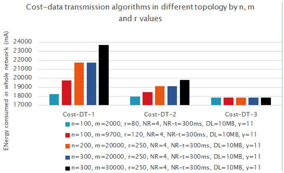
Cost of data transmission algorithms in different n, m, and r values.

Figure 22.

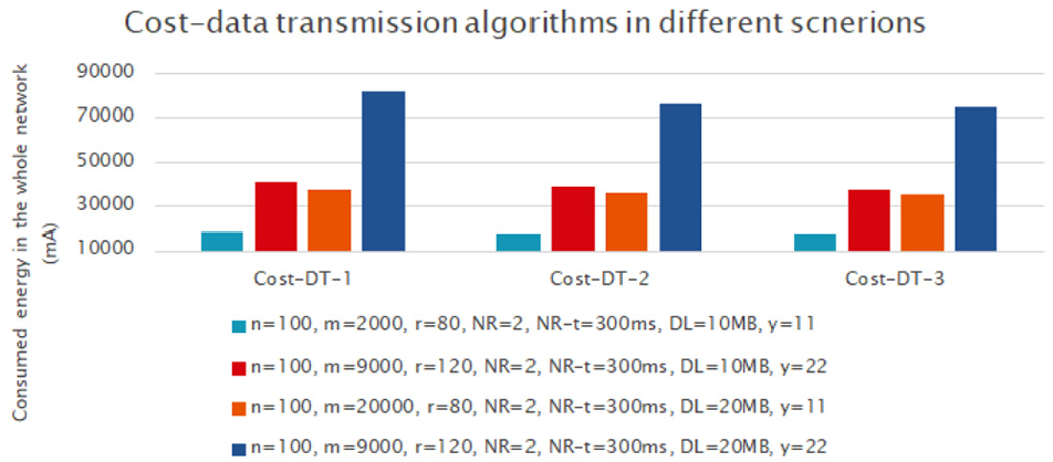
Cost of data transmission algorithms in different scenarios.

In first case, as shown in Figure 21, the amount of energy consumed to transmit 10 MB of data is examined for each of the three algorithms. According to the results yielded by the pathfinder algorithm, the most optimal route consists of 11 nodes. This is represented by y. In this case, NR and NR_t values are set to 4 and 300 ms, respectively. The constant behavior of the third algorithm shown by the graph in Figure 21 is due to the fact that the third algorithm does not call the pathfinder function at all, therefore, it is independent of n, r, and m parameters as depicted in equation (14). It depends on the number of nodes that are selected in the most optimal route by pathfinder function (y) and size of data (DL) only as shown in the equations (5) and (6). However, the performance of the other two algorithms is affected by all parameters. Because, the first and second algorithms are affected by the pathfinder algorithm.

As shown in Figure 22, DT₃ has various results because it is dependent on c and y parameters. In this case, NR, y, and DL are set to various values. In addition, as seen in the second and third scenarios of Figure 22, the m is as important as the data size (DL) in the energy consumption.

The following results were obtained by comparing the scenarios we have self-employed with a study in the literature ²⁴ that is shown in Figure 23. In this study, due to the evaluation of many parameters, the related studies were executed accordingly.

Figure 23.

Comparison cost of proposed data transmission algorithms and DDBL in different scenarios.

Conclusion and future works

In this article, a dynamic protocol was proposed to meet the needs of various applications. This protocol will be more efficient to use in IoT-based applications because it focuses on real-time large-data transmission. The proposed protocol consists of neighbor finding and creating routing tables, finding the best path, and data transmission algorithms. In this article, five algorithms were demonstrated. One of them is a neighbor finder algorithm. It calculates the cost from each node to all its neighbors and from that node to the BS. Therefore, each node can create its routing table at the end of the algorithm. The second algorithm is pathfinder proposed to find the possible routes and best path between the sender and target (destination) nodes in the network. This algorithm works more efficiently because each node can update its cost to target based on the information that it received from nodes in its layer before broadcasting a packet to its neighbors in contrast to many studies in the literature. It efficiently manages the power and the processor units. Therefore, it does not behave like greedy algorithms such as Dijkstra, and its success rate is higher to find optimized paths. In addition, three different algorithms were proposed for data transmission that can be applied in various scenarios and applications. The reason for the recommendation of three different mechanisms is to present a dynamic routing method and improve its applicability. The performances of all the proposed algorithms were evaluated theoretically and experimentally. In this study, we used the custom-manufactured sensor nodes, which were named KIANI-WSN kits.

In future works, we have a comprehensive roadmap part of which is shared here. We are planning to develop an application that will be used in our next studies by applying the relevant protocol to an agriculture and mining application. Also, we are planning to simulate a custom general framework software application, which can simulate all cross-overs in nodes by using the state-based model and plan to run adaptively on the relevant hardware, as a matter of fact this work has been started. On the contrary, the development and implementation of the dynamic data frame structure has been planned. In addition, we plan to develop a protocol that contains a learning feature by implementing nodes as an intelligent node by reinforcement learning-based methods such as learning automata and game theory techniques.