Sage Journals: Discover world-class research

Abstract

This article presents an image-based method to find the beam moment and shear force using the measured beam displacements. A least-squares method is first developed to find the rotations and lateral displacements at beam ends using the measured displacements along the beam. Then, the moments and shear forces of this beam segment are obtained using the matrix formulation including shear deformation and large displacement effects. Two experimental schemes, image symbol dot and image-correlation methods, were used to validate the accuracy of the proposed scheme. The comparison of the results between the finite element analysis and the two methods shows acceptable accuracy. Although this method is mainly applied to the elastic region, one can still find the moment and shear force at the inelastic region using the equilibrium equation.

Keywords

Computer image co-rotation digital camera displacement experiment finite element least-squares moment shear image-correlation method deflection

Introduction

In detailed inspections of structural safety, the moments and shear forces of bridge girders or building beams are often the important objects that should be measured. It seems that only the strain gage experiment can be used to measure beam moments directly, but this method often requires complicated installation procedures. Other experiments, such as Moiré, photoelasticity, and thermoelastic, can also be used to find the displacement or stress field of a body, but very few researches have presented how to evaluate beam moments and shear forces using those measured fields. Initial digital image-correlation concepts were presented by Sutton et al.¹ for displacement measurements, and the technique has been improved upon many times since. Korsunsky et al.² used the simplified beam-bending eigenstrain analysis of the residual elastic strains fields arising due to laser processing to optimize and characterize the approximate plastic strain profiles. Chu et al.³ developed a completely automated approach for computation of surface strains and displacements and later employed it to determine the centerline displacements of a cantilever beam. Lu and Cary⁴ developed the digital image-correlation method by implementing a second-order approximation of the displacement gradients and engaged it to measure more accurate displacement and strain. Baumann and Butefisch⁵ designed a Moiré interferometry system to acquire the instantaneous deformation of models during wind tunnel testing. The bending angle of a flap of a hypersonic vehicle was measured in their tests to determine the hinge moment due to aerodynamic loads. Barbero and Turk⁶ investigated the behavior of structures under combined axial load and moment experimentally. Their study used displacement transducers and full-field shadow Moiré to record all the deformation modes of the beam column. Hailstorm and Lundberg⁷ applied Timoshenko’s model for evaluation of shear force, transverse velocity, bending moment, and angular velocity at an arbitrary section from four independent measurements of such quantities at one to four sections. Razzaq et al.⁸ described an experimental and theoretical study of the flexural behavior of a commercially available thermoplastic beam subjected to a gradually increasing midspan concentrated load. The study was used to outline simplified criteria for a load and resistance factor design (LRFD) approach. Jia et al.⁹ proposed the six-axis heavy force sensor based on the Stewart platform fixed to a load sharing beam for the measurement of a multi-axis heavy force. Meng et al.¹⁰ describe an experimental study of a skew bridge to validate a finite element model. Results for static displacements, natural frequencies, mode shapes, and damping of the model bridge were presented in their experiments and finite element analyses, and a comparison of the results showed that good correlation was obtained. Lin et al.¹¹ developed a method for interpretation of lateral pile-load test results via measured inclinometer data. The study used the Fourier series function to represent the deflection behavior of the pile-soil system and obtained the shear, moment, and soil reaction along the pile shaft. Psimoulis and Stiros¹² used the robotic total station (RTS) to measure the oscillations and deflections of bridge girders. They indicated that the least-squares-based software can extend the range of application of RTS to higher frequency oscillations. Yoneyama et al.¹³ applied the digital image-correlation method into deflection measurement of real bridge during the bridge load testing, but beam shear force and moment were not determined in their paper. Chakrabarti et al.¹⁴ developed a nonlinear finite element model for the analysis of plain and reinforced concrete (RC) column confined by fiber-reinforced polymer (FRP) sheets. The study was based on appropriate selection of elements and strength failure criteria required for accurate analysis of concrete columns confined with FRP sheets. Charuchaimontri et al.¹⁵ performed a full-scale test on three RC long span link slabs to validate their finite element model, which can be used to predict the effective moment of inertia of the link slab under midspan loading, end rotation, and end translation for the development of design criteria for a link slab. Destrebecq et al.¹⁶ investigated the actual mechanical behavior of a full-scale RC beam using a digital-image-correlation technique. In their study, the displacement fields derived from digital images captured are analyzed into crack detection and measurement. Due to its good resolution, the method is suitable for early crack detection and measurement. Mirzazadeh and Green¹⁷ used digital image correlation and fiber optic strain sensors to measure crack widths, deflections, and strains for large-scale RC beams tested at room and low temperature. The study also conducted the calibration tests to measure the temperature-related strains induced in these systems. Wang¹⁸ presented a technique for noncontact optical measurement of in-plane displacement based on correlation analysis to identify the position of a marker before and after deformation of a specimen or plane test object, and this method is simpler than other optical techniques in experimental processing and can be efficiently used to measure large deformations.

In the finite element and experimental methods, both rotations and displacements of beams are obtained first in order to find their moments and shear forces. However, there is no standard procedure to evaluate them only using lateral beam displacements without rotations. To the best of our knowledge, the research of this topic is limited in the literature, especially for a beam with large deformation and shear effect. This article evaluates beam moments and shear forces using the measured lateral displacements, which can be obtained using any experimental method, such as digital-image-correlation or direct measurement methods. In this study, an image-based digital-camera experiment was used to find the lateral displacements of beams without contacting them. The equipment required is only a commercial digital camera and a personal computer, with no need for extra illumination or vibration isolation.

Algorithm to calculate beam moments and shear forces

In this section, a least-squares method and the Timoshenko beam theory are adopted to evaluate beam moments and shear forces under the conditions of small strain, large rotation, and elastic material.

The main purpose of this section is to generate the rotations and lateral deflections at the two edges of a straight beam segment using the displacements that are measured along this beam segment. The Timoshenko beam theory is adopted in the derivation of the beam rotation as follows

θ = \frac{d w}{d x} - β = α - β

(1)

where w is the beam’s lateral deflection, $β$ is a constant shearing strain across the section, $α = dw / dx$ is the total rotation of the plane originally normal to the neutral axis of the beam, x is the beam neutral axis, and is the rotation of the tangent to the neutral axis. For a small-rotation problem, the lateral deflection w can be directly measured from the displacement normal to the neutral axis of the original beam segment. For a large-rotation problem, the normal (dy_i) and axial (dx_i) displacements of the original beam at point i are measured first, and then, the co-rotational method is applied to find the lateral displacements (w_i) under the coordinates of the deformed beam. As shown in Figure 1(a), if there are m measured points of this beam segment ((dx_i, dy_i), i = 1, m), where points 1 and m are located at the beginning and end of the beam segments, respectively, the lateral displacements (w_i) are calculated as follows

\begin{matrix} {\begin{matrix} u_{i} \\ w_{i} \end{matrix}} = [\begin{matrix} \cos λ & \sin λ \\ - \sin λ & \cos λ \end{matrix}] \\ ({\begin{matrix} d x_{i} \\ d y_{i} \end{matrix}} - (1 - t) {\begin{matrix} d x_{1} \\ d y_{1} \end{matrix}} - t {\begin{matrix} d x_{m} \\ d y_{m} \end{matrix}}) \end{matrix}

(2)

where u_i is the axial displacement at point i, w_i is the lateral displacement at point i, $\sin λ = (d y_{m} - d y_{1}) / L$ , $\cos λ = (L_{0} + d x_{m} - d x_{1}) / L$ , L₀ is the original length, L is the current length $(L = \sqrt{{(L_{0} + d x_{m} - d x_{1})}^{2} + {(d y_{m} - d y_{1})}^{2}})$ , t = (X_i − X₁)/L₀, and X_i and X₁ are the X-coordinates at points i and 1, as shown in Figure 1(a).

Figure 1.

Co-rotation method to find beam nodal rotations: (a) coordinate transformation and (b) details of the beam element with two edge nodes.

For a beam element with two edge nodes labeled as 1 and m (Figure 1(b)), lateral deflection w_i at measured point i within this element can be interpolated using the Hermitian shape functions as follows

w_{i} = [\begin{matrix} N_{1}^{i} & N_{2}^{i} & N_{3}^{i} & N_{4}^{i} \end{matrix}] {[\begin{matrix} v_{1} & α_{1} & v_{m} & α_{m} \end{matrix}]}^{T} = {[N]}_{i} {u_{b}}

(3)

where

\begin{matrix} [N]_{i} & = [\begin{matrix} N_{1}^{i} & N_{2}^{i} & N_{3}^{i} & N_{4}^{i} \end{matrix}] \\ = [\begin{matrix} {(1 - r)}^{2} (2 + r) / 4 & (1 - r^{2}) (1 - r) L / 8 & {(1 + r)}^{2} (2 - r) / 4 & (r^{2} - 1) (1 + r) L / 8 \end{matrix}] \end{matrix}

(4)

and {u_b} is the nodal displacement vector, and it is given as

{u_{b}} = {[\begin{matrix} v_{1} & α_{1} & v_{m} & α_{m} \end{matrix}]}^{T}

(5)

where L is the element length, r = –1 + (2x_i − x₁)/L is the nondimensional coordinate, x₁ is the nodal coordinate at node 1, and x_i is the coordinate at the measured point i, as shown in Figure 1(b). It is noted that w₁ and w_m are zero after calculating from equation (2), so v₁ and v_m are also near zero.

The lateral deflections (w_i, i = 1, m) at m points along the deformed beam element can be calculated using equation (1), and one can also calculate the values of the shape function ([N]_i, i = 1, m) at each measured point using equation (4). Thus, the following least-squares method is able to evaluate the nodal displacement vector

{u_{b}} = [S] {F}

(6)

where

[S] = \sum_{i = 1}^{m} {[N]}_{i}^{T} {[N]}_{i} and {F} = \sum_{i = 1}^{m} {[N]}_{i}^{T} w_{i}

(7)

It is noted that the number of lateral displacements m must be larger than or equal to 4, or there are insufficient known values to solve equation (7).

To calculate beam moments and shear forces, a plane, straight, prismatic beam with two nodes is considered. The element is assumed to be initially aligned with the x-axis (Figure 1(a) and (b)). The local or co-rotated coordinate system $(\hat{x} - \hat{y})$ for the beam element is attached to the element and defined so that the $\hat{x}$ -axis remains coincident with a line joining the end points of the element, as shown in Figure 1(b). Thus, two nodal lateral deflections are zero in the local coordinate system, and two local nodal rotations are

{\hat{θ}} = {\begin{matrix} {\hat{θ}}_{1} \\ {\hat{θ}}_{2} \end{matrix}} = {\begin{matrix} θ_{1} - ϕ \\ θ_{2} - ϕ \end{matrix}}

(8)

where quantities with a “hat” will be used throughout this work to denote quantities measured in the co-rotated coordinate system and $ϕ = \sin^{- 1} [(v_{m} - v_{1}) / L]$ . It is noted that $ϕ$ is near zero due to the coordinate transformation of equation (2).

The relationship between nodal moments and nodal rotations can be found using the following matrix equation that includes shear deformation

{{\hat{M}}^{1}} = [K] {\hat{θ})

(9)

{\hat{M}} = {{\hat{M}}^{1}} + {{\hat{M}}^{0}}

(10)

where ${\hat{M}} = {\begin{matrix} {\hat{M}}_{1} \\ {\hat{M}}_{2} \end{matrix}}$ is the nodal moment vector, ${{\hat{M}}^{0}} = {\begin{matrix} {\hat{M}}_{1}^{0} \\ {\hat{M}}_{2}^{0} \end{matrix}}$ , is the fixed-end moment vector, and ${{\hat{M}}^{1}} = {\begin{matrix} {\hat{M}}_{1}^{1} \\ {\hat{M}}_{2}^{1} \end{matrix}}$ is the nodal moment vector without adding the fixed-end moments

[K] = \frac{1}{1 + b} [\begin{matrix} \frac{(4 + b) EI}{L} & \frac{(2 - b) EI}{L} \\ \frac{(2 - b) EI}{L} & \frac{(4 + b) EI}{L} \end{matrix}]

(11)

$b = 12 EI / L^{2} G A_{v}$ , E is Young’s modulus, G is the shear modulus, I is the moment of inertia, A_v is the shear area, and L is the beam current length.

From equation (1), the nodal rotations can be arranged as follows

{\hat{θ}} = {\hat{α}} - {\hat{β}} = {\hat{α}} - \frac{1}{G A_{s}} {\hat{V}}

(12)

where ${\hat{α}} = {\begin{matrix} {\hat{α}}_{1} \\ {\hat{α}}_{2} \end{matrix}}$ is the total rotation vector generated by equation (6), ${\hat{β}} = {\begin{matrix} {\hat{β}}_{1} \\ {\hat{β}}_{2} \end{matrix}}$ is the shear rotation vector, and ${\hat{V}} = {\begin{matrix} - {\hat{V}}_{1} \\ {\hat{V}}_{2} \end{matrix}}$ is the nodal shear vector.

The relationship between nodal moments and nodal shear forces is

{\hat{V}} = [R] {{\hat{M}}^{1}} + {{\hat{V}}^{0}}

(13)

where $[R] = \frac{- 1}{L} [\begin{matrix} 1 & 1 \\ 1 & 1 \end{matrix}]$ is the transformation matrix and ${{\hat{V}}^{0}} = {\begin{matrix} - {\hat{V}}_{1}^{0} \\ {\hat{V}}_{2}^{0} \end{matrix}}$ is the fixed-end shear force vector.

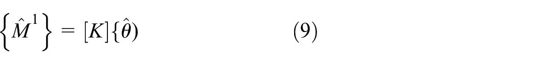
Substituting equations (12) and (13) into equation (9), one obtains the following equation

{{\hat{M}}^{1}} = {([I] + \frac{1}{G A_{s}} [K] [R])}^{- 1} ([K] {\hat{α}} - \frac{1}{G A_{s}} [K] {{\hat{V}}^{0}})

(14)

The nodal moment and shear force vectors can then be obtained using equations (10) and (13). These moments or shear forces will not be exactly equal when they are calculated from two sides of a node. The difference is dependent on the accuracy of the least-squares results using equation (6), and the error may be large for a large-rotation problem. An alternative scheme is to average the nodal moments calculated from the two sides of a node, and the nodal shear forces are then evaluated from equation (13) using these averaged nodal moments.

Theoretical and numerical validations

Theoretical and numerical simulations were conducted initially in this part to assess the computational reliability and robustness of the method. These simulations used theoretical or finite-element-predicted experimental input values of displacements dx_i and dy_i for equation (2).

A simply supported beam subjected to a uniform load

For a simply supported beam subjected to a uniform load (S), the theoretical solution of the beam lateral deflection (dy(x)) using the energy method for the small displacement and linear elastic assumption is

dy (x) = \frac{Sx}{24 EI} (L^{3} - 2 L x^{2} + x^{3}) + \frac{x (L - x)}{2 G A_{s}}

(15)

where L is the beam length and x is the distance from the left end of the beam. The beam is a rectangular section with the width and depth of 0.5 and 1 m, respectively. The beam length (= 1 m) over the beam depth is set to 1, so the shear deformation is dominant (over 70% of the total lateral deformation). The shear area A_s is 0.4167 m², Young’s modulus is 200 GPa, and the shear modulus is 80 GPa.

To find beam moments and shear forces, the simply supported beam is divided into n equal-length elements. Along each element, equation (15) is used to generate m lateral deflections with equal intervals from the beginning and end of each element, and these deflections are used to simulate the experimental results. Equation (6) is then adopted to find nodal rotations and lateral deflections of the element. Finally, equations (14), (10), and (13) are used to find the nodal moments and shear forces of each beam element. The calculated moment and shear force are normalized by the maximum moment at the beam center and the maximum shear force at the beam end as follows

M_{n} = \frac{M}{(S L^{2} / 8)} and V_{n} = \frac{V}{(SL / 2)}

(16)

where M and V are the calculated beam moment and shear force using equations (13) and (10), respectively; S is the uniform load; and L is the total beam length.

Figure 2 shows the beam moment and shear force diagrams using the theoretical and proposed methods. Figure 2 indicates that only when the simple beam is divided into two elements (n = 2), there is a small error for the moment diagram. Otherwise, the two methods provide very similar results that are almost independent of the variation of n (the number of elements) and m (the number of lateral displacements in an element). Thus, the proposed method can be used to evaluate beam moments and shear forces accurately, even for beams with a large portion of shear deformation.

Figure 2.

(a) Moment and (b) shear diagrams from theoretical and proposed methods (n = the number of elements and m = the number of lateral displacements in an element).

A simply supported beam subjected to a large concentrated force at beam center

The example is a simply supported beam subjected to a concentrated force (F) at the beam center, where the force is sufficiently large to produce a finite rotation of the beam, but the material is still within the elastic range. The simple beam section and material properties are as follows: rectangular section with the dimensions of 1 × 1 m², beam length L of 30 m, shear area A_s of 0.8333 m², Young’s modulus of 200 GPa, shear modulus of 76.92 GPa, and Poisson’s ratio of 0.3. The beam lateral deflection (w(x)) was calculated using a finite element code¹⁹ under the updated Lagrange formulation and the plane-stress assumption within the elastic range. Figure 3 shows the finite element mesh modeled by eight-node isoparametric elements and the deformed beam under F of 2 × 10⁶ kN.

Figure 3.

Finite element mesh and a deformed figure of a simple beam in example 2 (E = 200 GPa, v = 0.3, F = 2 × 10⁶ kN, beam length = 30 m, and beam section = 1 × 1 m).

In the finite element mesh along the beam centerline, the simply supported beam is divided into 361 nodes whose lateral deflections are used to simulate the experimental results. To find beam moments and shear forces, each beam segment is defined as containing m nodal lateral deflections, and equation (6) is adopted to find the rotations and lateral deflections at the two ends of the element. Finally, equations (14), (10), and (13) are used to find the nodal moments and shear forces of each beam segment.

Figure 4 shows the beam moment and shear force diagrams using the finite element and proposed methods, where the horizontal axis of Figure 4 is the current horizontal coordinates of the deformed beam. The calculated moments and shear forces near the applied concentrated force have large errors. This is because the displacement field at the applied force is singular and causes a complicated displacement distribution near this singular point; thus, the calculated moments and shear forces near this point are not shown in Figure 4. Usually, the displacement field can be normal about two section depths away from the singular point. Otherwise, Figure 4 indicates that the two methods obtain very similar results. Thus, the proposed method can be used to evaluate beam moments and shear forces for a large displacement problem.

Figure 4.

(a) Moment and (b) shear diagrams from finite element and proposed methods (m is the number of lateral displacements in an element).

Explanation of digital-camera experiment

In this study, there are two experimental methods, image symbol dot and image-correlation methods, to measure the displacements. The two methods have the same setup of the experiment, and only the pattern in the specimen is different. The experiment setup is shown in Figure 5, where the applied loading is given by the 100-kN Instron-8800 servo-hydraulic testing machine and a digital camera on a tripod is used to take the images of the specimen through a personal computer. The experiment is similar to that of Ju et al.,²⁰ but a normal camera lens is used to replace the microscope on the digital camera. The following sections illustrate the digital-camera experiment used in this study.

Figure 5.

Details of the experimental setup.

Description of optical system and specimens

The optical system is a Canon EOS 1D Mark II digital camera (with 4992 × 3328-pixel maximum resolution) with a Nikon AF 28-80-mm camera lens mounted on a standard tripod. The camera is controlled by shooting software with the shutter speed of 1/125 s, the ISO of 200, and the automatic setting of diaphragm and focus. The image is stored in an uncompressed TIFF file.

The specimen used in the digital-camera experiments is a square frame with the dimensions as shown in Figure 6. The four rectangular members of the specimen have the cross section of 45 × 6 mm, where the width of 6 mm is in the plane of the frame. The material is A36 steel with Young’s modulus of 215 GPa and Poisson’s ratio of 0.29. For the image symbol dot method, a marking pattern (306 mm long and 6 mm wide) was printed with black ink dot symbols on a laser printer (600 dpi resolution), as shown in Figure 6. For the image-correlation method, the random pattern was produced on the surface of the specimen to measure displacement (Figure 7). This kind of pattern could be obtained by first painting white paint and over-spraying with a mist of black paint.

Figure 6.

Details of the dimensions and specimen shape with dot symbols.

Figure 7.

Procedure of making random pattern for the image-correlation method: (a) painting white paint on specimen and (b) over-spraying black mist paint on specimen.

Experimental procedures

The specimen is mounted on the Instron-8800 testing machine with the vertical applied displacements between points a and c of Figure 6. The applied displacements to the specimen contain four steps of 0, 2, 4, and 7 mm for the image symbol dot method and three steps of 0, 2, and 7 mm for the image-correlation method. The digital camera captured images in sequence at each displacement stage and took the first image under the zero loads as a reference image for deflection calculation. The complete assembly was placed on a concrete floor in general conditions. Except for the normal lighting in the laboratory, there was no extra illumination; moreover, no arrangement was made to isolate ambient vibrations during the experiment.

Computer image analysis system

There are two Fortran programs to determine the displacement. One is CCD9 for the image symbol dot method and the other is CCD76 for the image-correlation method. The two programs can be obtained from the web (http://myweb.ncku.edu.tw/∼juju).

CCD9

The procedure for measuring displacement by the algorithm can be summarized as follows:

Subroutine RIMAGE (about 120 statements): it reads the TIFF file and obtains the red, green and blue (RGB) values at each pixel for a total of 4992 × 3328 pixels.

Subroutine GP (about 100 statements): based on the RGB array, it finds the region occupied by each dot symbol, which is similar to the polygon-filling in computer graphics. It is noted that the R = G = B = 0 for pixels representing the stickers and black dot symbols are significantly different from the reading for pixels in other parts of the image. The program can find regions containing pixels that have similar RGB values to the dot symbol, but since the size of a dot symbol is known, regions that are too large or too small are designated noises and skipped. The calculation result from the program is shown in Figure 8.

Subroutine GPX (about 100 statements): it calculates the center coordinates of each dot region. The displacement at each dot in each load stage is determined by deducting the deformed pixel coordinates from those of the zero-load case. The deformation counted by pixels is then converted to the physical deformation by a scale factor.

Figure 8.

Image from the CCD3 program under applied displacements of 0 and 4 mm to the specimen.

CCD76

The method for comparing two subsets is commonly given by use of the cross-correlation coefficient C as follows³

\begin{matrix} C (x, y, u, v, \frac{\partial u}{\partial x}, \frac{\partial u}{\partial y}, \frac{\partial v}{\partial x}, \frac{\partial v}{\partial y}) \\ = \frac{\sum [f (x, y) \cdot g (x^{*}, y^{*})]}{{[\sum (f {(x, y)}^{2} \cdot g {(x^{*}, y^{*})}^{2})]}^{1 / 12 2}} \end{matrix}

(17)

where f(x, y) are undeformed subset intensity values at selected points within the subset and g(x*, y*) are deformed subset intensity values at selected points within the subset

x^{*} = x + u + \frac{\partial u}{\partial x} Δ x + \frac{\partial u}{\partial y} Δ y

(18)

y^{*} = y + v + \frac{\partial v}{\partial x} Δ x + \frac{\partial v}{\partial y} Δ y

(19)

where x is the center point x-direction coordinate of subset; y is the center point y-direction coordinate of subset; u is the center point x-direction displacement; v is the center point y-direction displacement; $du / dx$ , $du / dy$ , $dv / dx$ , and $dv / dy$ are derivative terms at center point; Δx is the chosen point x-direction distance from center point; and Δy is the chosen point y-direction distance from center point. The image-correlation method may lose accuracy if the number of subsets in a certain direction is not enough to evaluate precise displacement derivatives, such as the transverse direction of a slender beam.

After the experiment, the undeformed and deformed TIFF image files were then processed by the PC-based program named CCD76 (http://myweb.ncku.edu.tw/∼juju). The FORTRAN program used the image-correlation method to find the displacements and strains of the square blocks divided in the image. The procedures of the program are illustrated as follows:

Subroutine RIMAGE (about 120 statements): It reads the TIFF file and obtains the red, green, and blue (RGB) values at each pixel for a total of 4992 × 3328 pixels.

Subroutine GetGray (about 10 statements): It transfers the RGB values at each pixel to gray level value. The transforming equation =R×0.299+G × 0.587+B × 0.114, where R, G, and B are the red, green, and blue values of the image.

Subroutine Getuv (about 83 statements): When the displacement range and increment are selected, use linear search method to find the most correct u and v displacements of each square block at the highest cross-correlation value. The gray values of undeformed and deformed blocks are obtained from subroutines Fdo and FdDisp, and equation (17) is applied to obtain the cross-correlation value.

Subroutine Fdo (about 23 statements): it finds the n × n array of the gray values of the undeformed square block, in which n is the number of pixels of the block side.

Subroutine FdDisp (about 47 statements): it finds the n × n gray values of the deformed block, which is not necessary to be a square block as the undeformed one. The pixel coordinates x* and y* in this deformed block using equations (18) and (19) may be not integer values, so the bilinear interpolation is applied to approximate the gray-level value at the point (x*, y*).

Subroutine duvxy (about 47 statements): this subroutine applies the central difference method to obtain the differential information of $du / dx$ , $du / dy$ , $dv / dx$ , and $dv / dy$ .

Experimental accuracy due to ambient vibrations

Because optical experiments often have a rigorous requirement for ambient vibrations, this section investigates the experimental error caused by these vibrations in the laboratory. The previous section shows that deflections are calculated by two pictures under zero and a specific applied load, so the error of each picture will not be spread to other pictures. The maximum error (Error_pixel) of pixels during taking a picture can be estimated as follows

Erro r_{pixel} = \frac{S_{shutter} V_{vibration}}{P_{scale}}

(20)

where S_shutter (= 1/125 s used in this study) is the shutter speed of the digital camera, V_vibration (mm/s) is the maximum vibration velocity on the laboratory, and P_scale (about 0.06 mm/pixel used in this study) is the resolution of the pictures. During the laboratory experiments, three velocity meters were installed on the Instron machine to measure vibrations in three directions, and they obtained the maximum vibration velocity (V_vibration) of 0.05 mm/s. Thus, Error_pixel equals 0.007 pixel, which is a very small error and will not produce inaccuracy in the digital-camera experiment.

Experimental results and comparisons

In this section, the finite element code¹⁹ was used to investigate the accuracy of the experimental result. The specimen was modeled by the two-node beam elements with the co-rotational method, where the connection regions of the specimen contain 0.5 cm rigid zones, and the beam element length was 0.612 cm. The following two sections illustrate the comparison results of the two methods.

Image symbol dot method

For the specimen, as shown in Figure 6, there are 49 symbols on member a–c of the frame, in which the diameter and interval of the black circular symbols on the specimen are 3 and 6 mm, respectively. Figure 8 shows the symbol positions under 0 and 1 mm applied displacement, and the displacements of symbols are the difference of the symbol coordinates between the two figures. The deformation counted by pixels is then converted to the physical deformation by a scale factor of 0.0065 mm per pixel, which was determined based on the image of the zero load. Figure 9 shows the lateral displacements of member a-c obtained from the finite element analysis (FEA) and the charge-coupled device (CCD) experiment, which indicates a good agreement between the finite element and experimental methods. In the CCD experiment, 23 displacements were used in the least-squares method to find moments and shear forces. At the first step, the displacements at the first 23 symbols were used to find the moments and shear forces at the locations of symbols 1 and 23. The second step shifted a symbol to find the moment and shear forces at symbols 2 and 24, and this continued until the moments and shear forces at symbols 27 and 49 were obtained in the last step. Figure 10 shows the moment and shear force distributions along member a-c obtained from FEA and the CCD experiment. Figure 10 shows that the accuracy of the comparison is acceptable.

Figure 9.

Comparison of deflections between experimental and finite element results.

Figure 10.

(a) Moment and (b) shear diagrams from finite element and image symbol dot methods.

If fewer than 23 displacements were used in the least-squares method to find moments and shear forces, the accuracy of the least-squares method will decrease. Since the moments are twice the differentiation of beam lateral deflections, a small variation of beam deflections may cause a large error in calculation of the moment. To overcome this problem, a higher definition digital camera should be used.

Image-correlation method

There are 229 blocks along the horizontal direction and 2 blocks along the vertical direction on the target member of the frame. The deformation obtained from the CCD76 program is pixels. It is necessary to convert the pixel deformation to the physical deformation by a scale factor of 0.0677 mm per pixel in this study. Figure 9 shows the lateral displacements of the target member (Figure 6) obtained from the FEA and the CCD experiment, which indicates a very good agreement between the two methods.

In order to determinate shear force and moment along the target member, 115 displacement data were adopted to find moments and shear forces using the least-squares method. Figure 11 shows the moment and shear force distributions along the target member obtained from the FEA and the CCD experiments under the applied displacements of 7 and 2 mm, respectively. These figures show that the accuracy of the comparison is acceptable using the image-correlation method. Moreover, Figures 10 and 11 show that both the image symbol dot method and image-correlation method can use the displacement field of the beam to obtain accurate moments and shears.

Figure 11.

(a) Moment and (b) shear diagrams from finite element and image-correlation methods.

Conclusion

This article presents a systematic method to find beam moments and shear forces using the measured beam displacements within the elastic range. First, a number of beam displacements are measured by an experimental method, such as computer image scheme of this study. Then, these displacements are substituted into a least-squares method with the co-rotation scheme to find the nodal rotations and lateral displacements at the two ends of a beam segment. Finally, beam moments and shear forces of this beam segment can be obtained using the matrix formulation including the shear deformation effect. Theoretical and numerical simulations indicate that the proposed method can be used to evaluate beam moments and shear forces accurately for problems dominated by shear deformation or large displacement effects. Using this method, one can calculate the moment and shear force at a certain section of a beam and then use the equilibrium equation to find moments and shear forces at other sections. Thus, although this method is mainly applied to the elastic region, one can still find the moment and shear force at the inelastic region using the equilibrium equation.

To measure the beam displacements, an image symbol dot and image-correlation methods were used in this article. The only equipment required is a commercial digital camera and a personal computer, with no need for extra illumination or vibration isolation. The above-mentioned image-based systems were used to measure the displacements of plane frames. Beam moments and shear forces were then evaluated by substituting these beam displacements into the proposed formulation. The comparison of the results between FEA and the current method shows an acceptable accuracy. Thus, one can use this experimental scheme and proposed formulations to measure the member moments and shear forces of bridges or buildings without contacting them.

Footnotes

Handling Editor: Daxu Zhang

Declaration of conflicting interests

The author(s) declared no potential conflicts of interest with respect to the research, authorship, and/or publication of this article.

Funding

The author(s) disclosed receipt of the following financial support for the research, authorship, and/or publication of this article: This study was supported by the National Science Council, Republic of China, under contract number NSC90-2218-E-006-063.

ORCID iD

Shen Haw Ju

References

Sutton

Wolters

Peters

et al . Determination of displacements using an improved digital correlation method. Image Vision Comput 1983; 1: 133–139.

Korsunsky

Vorster

WJJ

Zhang

et al . A beam-bending eigenstrain analysis of residual elastic strains in multi-scan laser-formed steel samples. Proc IMechE, Part C: J Mechanical Engineering Science 2008; 222: 1635–1645.

Chu

Ranson

Sutton

et al . Applications of digital-image-correlation techniques to experimental mechanics. Exper Mech 1985; 25: 232–244.

Cary

. Deformation measurements by digital image correlation: implementation of a second-order displacement gradient. Exper Mech 2000; 40: 393–400.

Baumann

Butefisch

. Measurement of hinge moments and model deformations in wind tunnels by means of Moiré interferometry. Soc Photo Opt Instru Eng 1995; 2546: 16–32.

Barbero

Turk

. Experimental investigation of beam-column behavior of pultruded structural shapes. J Reinforced Plastics Compo 2000; 19: 249–265.

Hillstrom

Lundberg

. Analysis of elastic flexural waves in non-uniform beams based on measurement of strains and accelerations. J Sound Vibra 2001; 247: 227–242.

Razzaq

Coskun

et al . Sampling Moiré, method for accurate small deformation distribution measurement. J Reinforced Plastics Compo 2009; 28: 2749–2759.

Jia

Lin

Liu

. Performance index analysis of a six-axis heavy force sensor based on the Stewart platform. Proc IMechE, Part C: J Mechanical Engineering Science 2010; 224: 1359–1368.

10.

Meng

Ghasemi

Lui

. Analytical and experimental study of a skew bridge model. Eng Struct 2004; 26: 1127–1142.

11.

Lin

Liao

Chen

et al . Lateral performance of piles evaluated via inclinometer data. Comput Geote 2005; 32: 411–421.

12.

Psimoulis

Stiros

. measurement of deflections and of oscillation frequencies of engineering structures using robotic theodolites (RTS). Eng Struct 2007; 29: 3312–3324.

13.

Yoneyama

Kitagwa

Iwata

et al . Bridge deflection measurement using digital image correlation. Exper Tech 2007; 31: 34–40.

14.

Chakrabarti

Chandra

Bharagava

. Finite element analysis of concrete columns confined with FRP sheets. J Reinforced Plastics Compo 2008; 27: 1349–1373.

15.

Charuchaimontri

Senjuntichai

Ozbolt

et al . Effect of lap reinforcement in link slabs of highway bridges. Eng Struc 2008; 30: 546–560.

16.

Destrebecq

J-F

Toussaint

Ferrier

. Analysis of cracks and deformations in a full scale reinforced concrete beam using a digital image correlation technique. Exper Mech 2011; 51: 879–890.

17.

Mirzazadeh

Green

. Fiber optic sensors and digital image correlation for measuring deformations in reinforced concrete beams. J Bridge Eng 2018; 23: 04017144.

18.

Wang

. Marker identification technique for deformation measurement. Adv Mech Eng 2015; 5: 246318.

19.

. Development a nonlinear finite element program with rigid link and contact element. NSC-86-2213-E-006-063, 1997, http://myweb.ncku.edu.tw/~juju

20.

Liu

. Measurement of stress intensity factors by digital camera. Int J Solids Struct 2006; 43: 1009–1022.