
Abstract
The main purpose of this article is to investigate the qualitative effects of different factors on the response of forced vibration of shape memory alloy spring oscillator. Specially, the introduction of dry friction factor causes the governing equations to change from a smooth system to a (Filippov-type) non-smooth system in which the sliding phenomenon was observed. The mechanism, geometric structure, and analytic conditions of sliding bifurcations in a general n-dimensional piecewise smooth system were discussed in detail. The theoretical results obtained are verified by numerical analysis, and the feasibility of involved theories is estimated by calculation of sliding time.
Introduction
Shape memory alloys (SMA) have been manufactured into intelligent and parameter-controllable components for deformation and vibration control of engineering structures and mechanical equipment due to their unique mechanical properties, such as shape memory effect and superelasticity. 1 SMA helical spring 2 is the most widely used SMA component. It has been used in automotive thermostat, gas pipeline fire valve, robot claw and overcurrent protector, and other devices as a driver. 3 At present, the researches on SMA spring mainly focus on its mechanical properties, deformation simulation, and design principle. 4 There are also some reports on the dynamic characteristics of SMA spring oscillator, 5 such as the response of the coupled SMA spring oscillator, 6 the nonlinear thermo-mechanical response of the single SMA spring oscillator,7,8 and the response of the non-smooth SMA spring oscillator. 9 However, the theoretical research on different comprehensive factors (temperature, damping, external excitation, dry friction, etc.) of the system is still lacking. It is worth mentioning that except for dry friction, other factors considered in this article will not change the smoothness10,11 of governing equations of the system. Therefore, new theoretical methods need to be found to study the effects of dry friction factor on the system.
In this article, the restoring force of SMA spring is described by the polynomial constitutive relation of SMA,12,13 and the nonlinear dynamic model of forced vibration of SMA spring oscillator is established. The response of the system is analyzed by means of bifurcation diagrams, Lyapunov exponent spectrums, time history diagrams, phase portraits, and Poincaré cross-sectional drawings. The bifurcation and chaos of this system are mainly discussed. The non-smooth differential equations with dry friction are discussed separately due to its particularity.
Restoring force model of SMA spring
The constitutive model of SMA proposed by Falk 14 is applied in this article. The constitutive equation of the model is

in which a, b, and e are material constants,

Therefore, the restoring force model of SMA spring can be established as

in which
Control equations for forced vibration of SMA spring oscillator
SMA spring oscillator system consists of a mass block with mass m, a linear damper with damping coefficient c, and the SMA spring. The mass block is subjected to harmonic excitation force

Forced vibration system of shape memory alloy (SMA) spring oscillator.
By Newton’s second law, the differential equation of vibration of the system can be expressed as

The dimensionless transformation can be written as follows

where


Formula (7) shows that the nonlinearity of the SMA material constitutive relation leads to the nonlinearity of the system state. The dynamic behaviors of the system are also affected by environmental temperature, damping, external exciting force, and other factors (such as dry friction), so the nonlinear dynamical response of the system is bound to be complex.
Numerical solution and analysis
Considering that the state equation of the system contains a quintic nonlinear term, the fourth-order Runge-Kutta method is used to solve the state equation of the system (7)

Assuming that the solution of the typical initial value problem (8) is
Runge-Kutta method is essentially a numerical method indirectly using Taylor series. For the difference quotient

Therefore,

In each step of the fourth-order Runge-Kutta method, the function value f has to be calculated four times, so its truncation error is lower while calculation accuracy is higher.
Nonlinear dynamical response of the system is analyzed by means of bifurcation diagrams, Lyapunov exponential spectrums, phase portraits, time history diagrams, and Poincaré cross-sectional drawings. In numerical simulations, the values of fixed relevant parameters are as follows

Influence of temperature on system response
In this case, the system parameters are shown in Table 1. When
Parameter table with varying


(a) The bifurcation diagram and (b) Lyapunov exponent spectrum with
Longitudinal coordinate X denotes dimensionless displacement, while
Lyapunov exponent can describe the motion characteristics of the system. It takes positive and negative values along a certain direction to indicate the average divergence or convergence rate of adjacent orbits along the direction of the system under the action of attractors for a long time. When Lyapunov exponent
It can be seen from Figure 2 that when
When
At bifurcation points
The phase portraits and Poincaré cross-sectional drawings of the system at two temperatures are presented in Figures 3 and 4 where ordinate Y represents dimensionless velocity. In the first case with
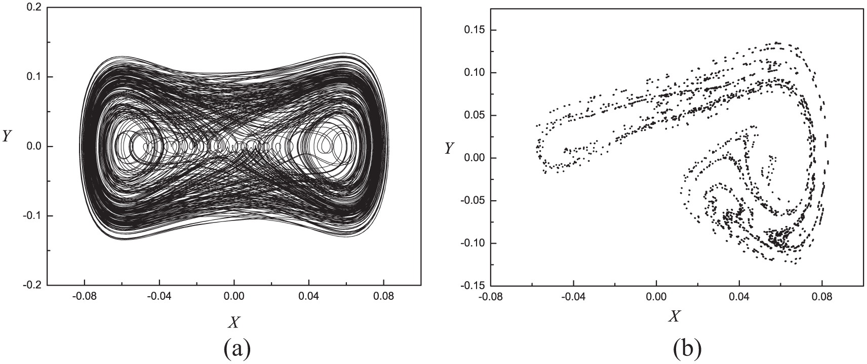
(a) The phase portrait and (b) Poincaré cross-sectional drawing with
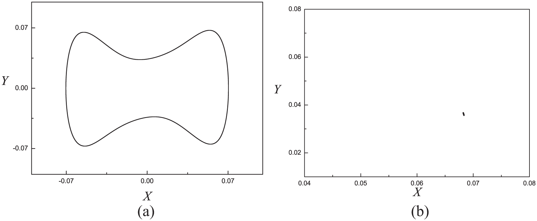
(a) The phase portrait and (b) Poincaré cross-sectional drawing with
When
Influence of damping coefficient on system response
In this case, the coefficients are shown in Table 2. When the amplitude of dimensionless excitation force is fixed at
Parameter table with varying

(a) The bifurcation diagram and (b) Lyapunov exponent spectrum with

(a) The bifurcation diagram and (b) Lyapunov exponent spectrum with

(a) The bifurcation diagram and (b) Lyapunov exponent spectrum with
It can be seen from the Figure 5 that the system is in chaotic motion at low temperature
Under the intermediate temperature state
When
When
Taking the medium temperature state as an example to verify the validity of bifurcation analysis results, the evolution of system trajectory is observed in detail. When

(a) The time history diagram, (b) phase portrait, and (c) Poincaré cross-sectional drawing with

(a) The time history diagram, (b) phase portrait, and (c) Poincaré cross-sectional drawing with
(a) The time history diagram, (b) phase portrait, and (c) Poincaré cross-sectional drawing with
(a) The time history diagram, (b) phase portrait, and (c) Poincaré cross-sectional drawing with
As shown in Figure 8, when
As shown in Figure 9, when
As shown in Figure 10, when
Influence of external excitation amplitude on system response
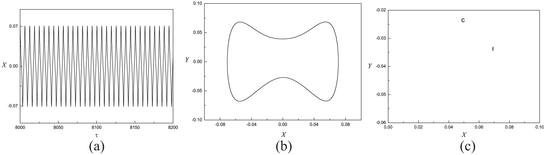
In this case, parameters are set as shown in Table 3. Figures 12–14 are the global bifurcation diagrams and Lyapunov exponent spectrums of the system varying with the amplitude H of the dimensionless exciting force. It can be seen that the coincidence degree between bifurcation diagram and exponential spectrum in the relevant interval is high.
Parameter table with varying H.


(a) The bifurcation diagram and (b) Lyapunov exponent spectrum with
(a) The bifurcation diagram and (b) Lyapunov exponent spectrum with
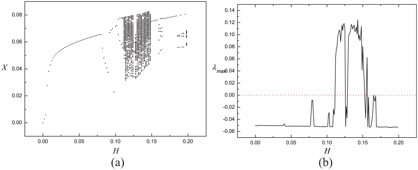
(a) The bifurcation diagram and (b) Lyapunov exponent spectrum with
It can be seen from the graphs that the motion of the system changes alternately between periodic motion and chaotic motion with the increase of H at any kind of temperature states. At different temperatures, corresponding periodic and chaotic motion intervals are different.
It is noteworthy that the displacement of the periodic motion jumps with the change of H, which is mainly caused by the selection of the initial value instead of bifurcation. Different initial point selection leads to the convergence of phase trajectories to different equilibrium states.
When

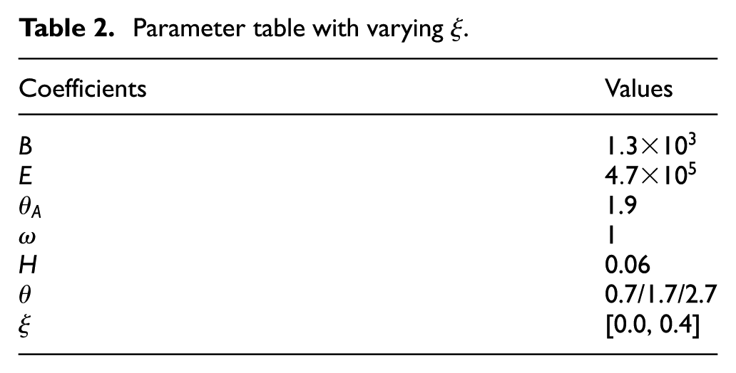
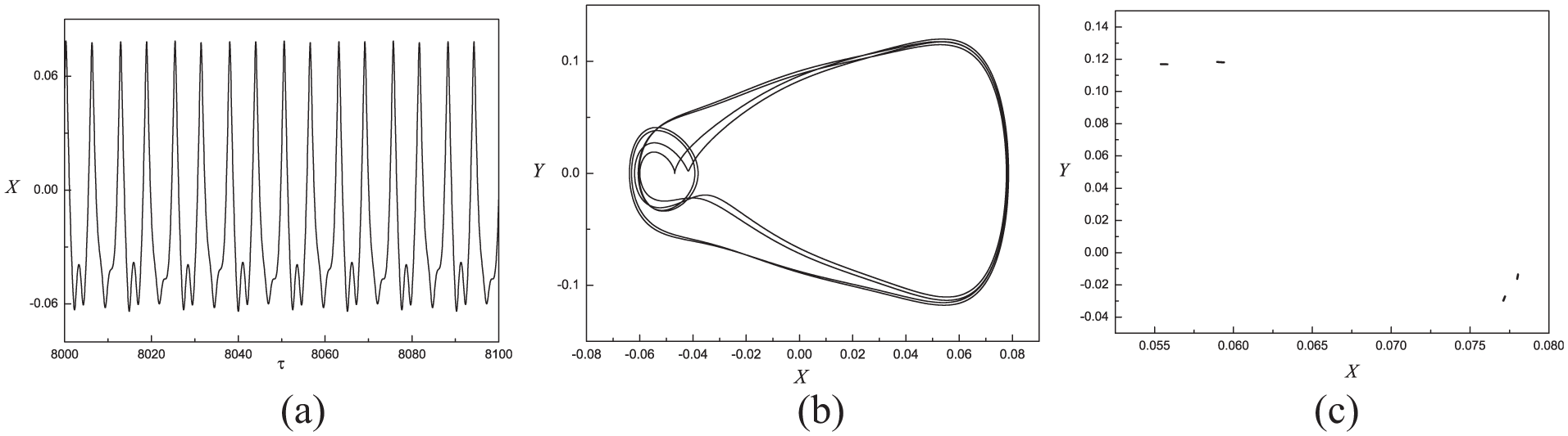
(a) The time history diagram, (b) phase portrait, and (c) Poincaré cross-sectional drawing with

(a) The time history diagram, (b) phase portrait, and (c) Poincaré cross-sectional drawing with
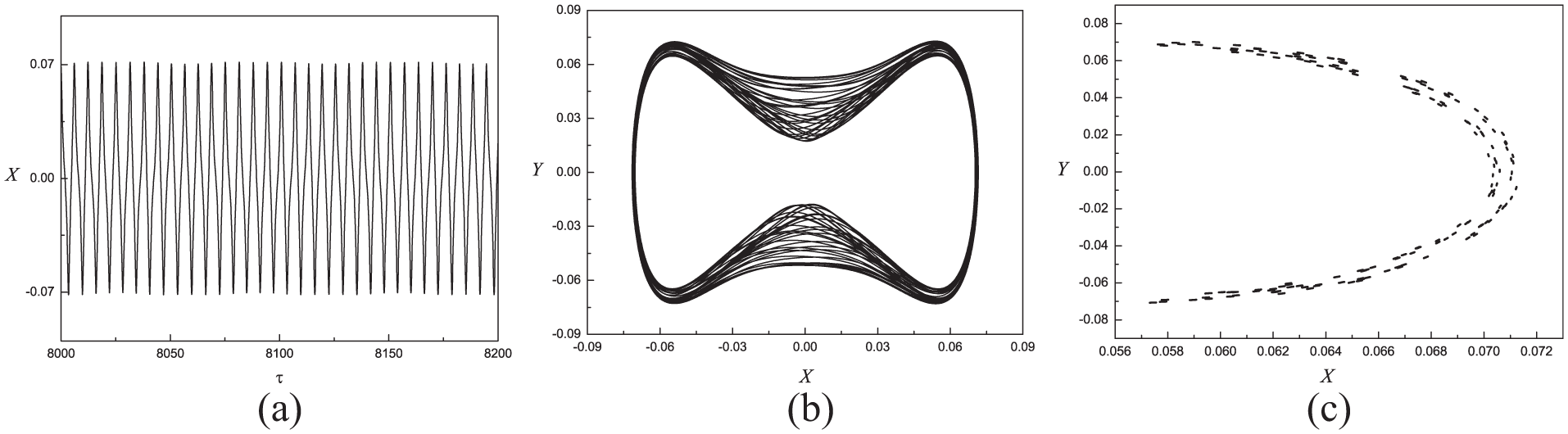
(a) The time history diagram, (b) phase portrait, and (c) Poincaré cross-sectional drawing with
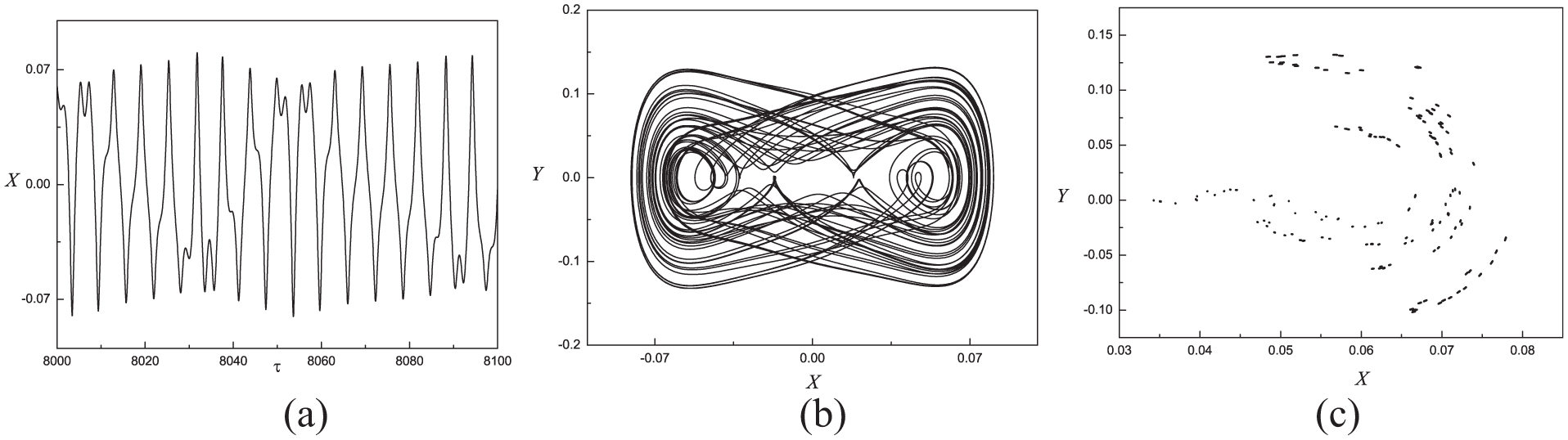
(a) The time history diagram, (b) phase portrait, and (c) Poincaré cross-sectional drawing with
It can be seen from Figure 15 that when
When
For the same reason, Figure 16 shows that system is in periodic-4 motion.
When
The motion characteristics of the system with different values of H can also be verified by the time history diagrams and phase portraits. Due to the article length limitation, it is omitted here.
Influence of dry friction factor on system response
To explore the mechanisms of non-smooth SMA oscillator,
15
a conveyer belt with a constant velocity

where

By the dimensionless transformation

the control equations can be described as
Through coordinate transformation

It is a typical Filippov system (piecewise smooth system).16,17 The parameters are set as shown in Table 4. The phase portraits are shown in Figure 19 where
Parameter table with varying H.

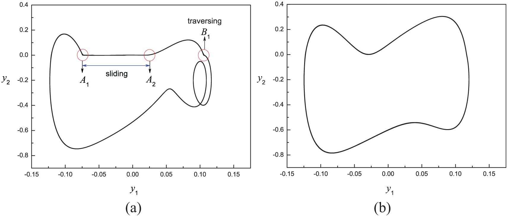
Phase portrait with (a)
Actually, in the engineering practice, the sliding (sticking) phenomenon is not always expected. For instance, the occurrence of sliding phenomenon of the lathes for producing molds with SMA spring means the production of defective products. 19 Therefore, finding out a way to eliminate the sliding phenomenon is of great concern. As shown in Figure 19(b), controlling the frequency of external excitation is a relatively simple and effective solution because the change of external excitation invalidates the necessary condition of sliding bifurcation which will be discussed in detail in the next subsection.
Because of discontinuity of the vector field resulting from
Mechanism and geometric structure of sliding bifurcation
Consider the general n-dimensional piecewise smooth system
The definition of the non-smooth boundary can be expressed as
in which

The specific expression of the sliding area and its boundary is


Taking the derivative of equation (21) with respect to Y, one may find that

For
There are four possible kinds of sliding bifurcation according to the way that the periodic solution of the system intersects with the boundary of the sliding region
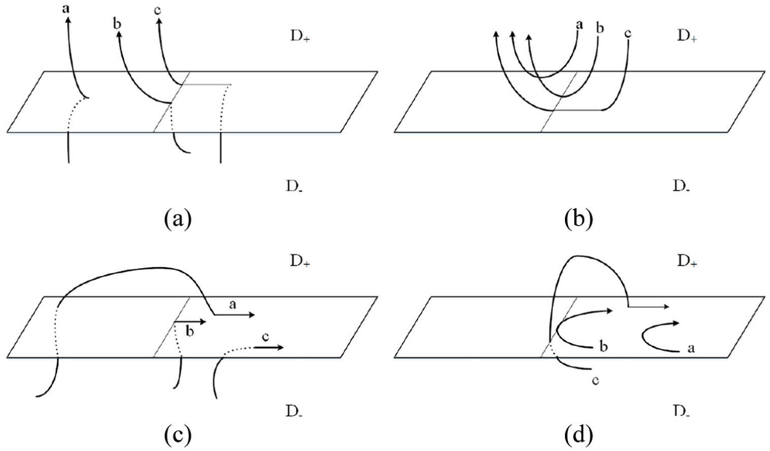
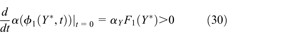
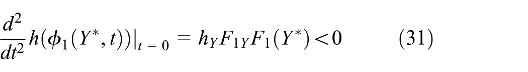
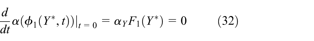
(a) The crossing sliding bifurcation, (b) The grazing sliding bifurcation, (c) The switching sliding bifurcation, and (d) The adding sliding bifurcation.
Figure 20(a) is used to describe the crossing sliding bifurcation. With the parameter varying, the trajectory traversed the boundary of the sliding region at the bifurcation point and left the sliding area (see trajectory b in Figure 20(a)). With further changes of parameters, the trajectory entered the sliding region, resulting in the appearance of sliding motion (see trajectory c in Figure 20(a)).
Figure 20(b) is the sketch map of grazing sliding bifurcation. 21 With the parameter varying, the trajectory is tangent across the boundary of the sliding region at the bifurcation point. (see trajectory b in Figure 20(b)). With the further changes of parameters, the trajectory entered the sliding region, resulting in the appearance of sliding motion (see trajectory c in Figure 20(b)).
Figure 20(c) shows the switching sliding bifurcation which is similar to the first kind of sliding bifurcation. The difference between them is that the trajectory remained in the sliding region after crossing the boundary of it (see trajectory b in Figure 20(c)). With further changes of parameters, a segment of the trajectory remained in the sliding region (see trajectory c in Figure 20(c)).
Figure 20(d) describes the adding bifurcation. The main difference between this bifurcation and the above three bifurcations is that the bifurcation trajectory of the system is completely located in the sliding region and tangent to the boundary of the sliding region at the bifurcation point (see trajectory b in Figure 20(d)). With further change of parameters, a segment of the trajectory was still in the sliding region (see trajectory c in Figure 20(d)).
Analytic conditions for sliding bifurcation
The four sliding bifurcations described in “Mechanism and geometric structure of sliding bifurcation” can be accurately described by analytical conditions which are given below.
1. The crossing sliding bifurcation and the grazing sliding bifurcation.
First, because the bifurcation point

Besides, the bifurcation point

where

By the law of derivation of the dot product and the combination of formulas (25), (27), and (28)

2. The switching sliding bifurcation.
It satisfies two basic conditions of equations (26), (27), and
3. The adding bifurcation.
It satisfies two basic conditions of equations (26) and (27). In this case, however, the bifurcation trajectory is completely located in the sliding region and is tangent to the boundary of it at the bifurcation point. Therefore
Besides, the bifurcation trajectory in this case has a minimum (The first-order derivative is equal to 0 while the second derivative is greater than 0.) at
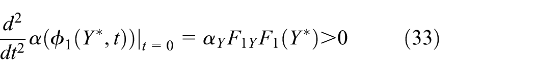
By the law of derivation of the dot product and the combination of formulas (25), (27), and (33)

With all the results obtained, it is easy to calculate the sliding region of the SMA spring oscillator as follows


where

where

So the sliding region can be described as

and the boundary of it can be written as


Numerical verification and discussion
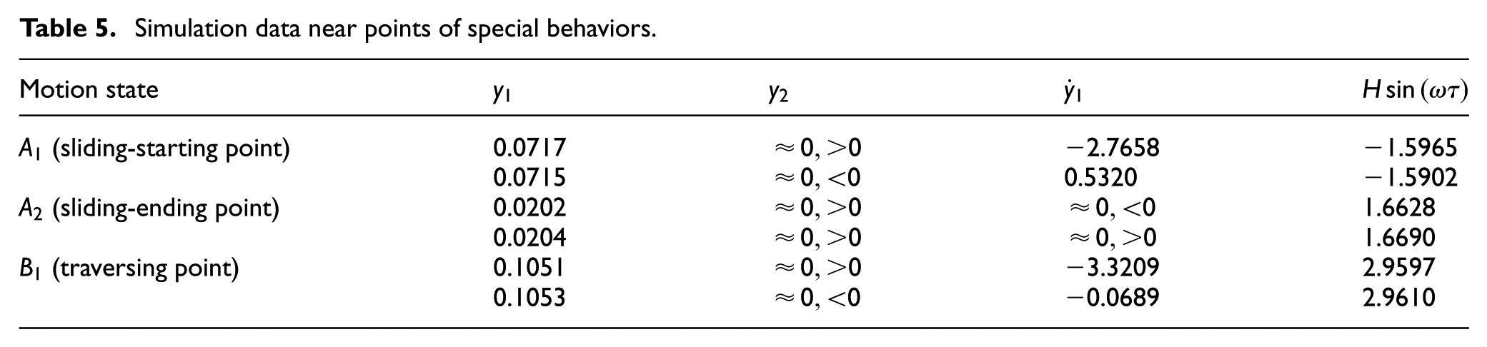
In order to better explore and understand the mechanism of sliding bifurcation, the sliding process in Figure 19(a) is numerically analyzed as follows, and the feasibility of the above theory is verified by calculating the sliding time.
It is noteworthy that at the starting point

(a) The structure of the vector field in sliding region and (b) The structure of the vector field in traversing region.
Sliding phenomena occur when there are opposite vector fields (
In addition, the sliding time can be estimated according to the variation of excitation
Simulation data near points of special behaviors.

Time history of
Conclusion
With the amplitude of exciting force and damping fixed at small values, periodic or chaotic motion can be observed with the temperature varying. When the amplitude of exciting force is fixed at a small value, with the increase of damping, chaotic, quasi-periodic, and periodic motion appear alternatively in the system. In the low temperature state
The introduction of dry friction factor changes the smoothness of the original system
In addition, this article only discusses the simple case in which dry friction is considered as a single variable temporarily. The coupling between dry friction and other factors will be discussed separately in other literatures.
Footnotes
Handling Editor: Yunn-Lin Hwang
Data Availability
All the data used to support the findings of this study are available from the corresponding author upon request.
Declaration of conflicting interests
The author(s) declared no potential conflicts of interest with respect to the research, authorship, and/or publication of this article.
Funding
The author(s) disclosed receipt of the following financial support for the research, authorship, and/or publication of this article: This research was supported by National Natural Science Foundation of China (Grant no. 11632008).