
Abstract
A hierarchical controller including a vehicle condition parameter estimator for improving the vehicle stability is theoretically applied to a four-wheel independent-drive electric vehicle. This study is aimed at combining the parameters estimation with vehicle stability control and evaluating different optimization algorithms based on the computation time and fluctuation. The hierarchical controller consists of a vehicle condition parameter estimator, active yaw moment controller, and torque distribution controller. The vehicle condition parameter estimator is based on the Unscented Kalman Filter, which avoids the truncation error caused by Taylor expansion to convert a nonlinear system into a linear system. The active yaw moment controller is designed based on the sliding mode control. The controller employs co-control between the vehicle sideslip angle and yaw rate, which properly accounts for both factors. The objective function of the torque distribution controller is based on the tire utilization function and constraint condition. The torque distribution and wheel slip rate are accounted for simultaneously. The torque distribution methods are tested based on nonlinear programming, quadratic programming, and weighted least squares for the sake of comparison. The simulation results demonstrate the accuracy of the proposed vehicle state estimator and the effectiveness of the proposed stability controller.
Keywords
Introduction
A four-wheel independent-drive (4WID) electric vehicle represents an innovative design in which four in-wheel motors are used to drive the wheels independently. The electric vehicle’s transmission efficiency is also improved because the conventional mechanical drive system is eliminated. The independent four-motor design also frees up interior space, is more conducive to wire-controlled applications, and allows a variety of novel control methods to be applied. 4WID electric vehicles can achieve electric power steering, differential drive assisted steering control, 1 electronic differentials, 2 energy regenerative braking, 3 and direct yaw moment control, 4 making the design extremely popular. 5
However, it is difficult to obtain the vehicle condition parameters directly through a sensor in a vehicle with a 4WID form; there is, therefore, currently a demand for novel vehicle state estimation algorithms suited to this purpose. Imslanda et al. 6 explored a new method for obtaining the longitudinal speed from the wheel speed and longitudinal acceleration in which the current state of the vehicle is initially determined, followed by a comprehensive calculation of the wheel speed and longitudinal acceleration by adjusting the weight coefficient to determine the vehicle speed. Hrgetic et al. 7 established another vehicle state (speed) estimation method using a nonlinear, adaptive extended Kalman filter (EKF). Li and Zhang 8 established another vehicle sideslip angle estimation method using a hybrid Kalman filter. However, the above researches did not apply the estimated results to the vehicle stability control. Therefore, the accuracy of the estimated state variables in vehicle control cannot be verified. On the contrary, general vehicle parameter estimation methods, such as EKF, are easy to introduce truncation errors in the estimation process.
There has been a significant amount of research to date on independent driving, electric vehicle stability control, and torque distribution. The available methods for solving the torque distribution issue include a generalized inverse method, 9 penalty function method, 10 chain increment method, and mathematical optimization method. Maeda et al. 11 investigated various independent-drive electric vehicle torque distribution strategies and built test prototypes to verify them; Li et al. 12 designed a yaw moment controller based on sliding mode control (SMC) and a torque distribution controller based on a penalty function. The above stability control methods of the vehicle are based on the assumption that the vehicle state has been obtained, and there are few studies comparing the computational time costs and fluctuation of different control methods.
In order to estimate vehicle parameters and verify the application of those parameters in vehicle stability control, the vehicle stability controller with parameter estimator is built. The Unscented Kalman Filter (UKF)–based estimation method avoids the effect of truncation error on the accuracy of results. The main aspects of this article are as follows: To solve the difficulty in obtaining the vehicle condition parameters of 4WID vehicles, this study establishes a hierarchical control system including a vehicle condition parameters estimator. In addition, the computational times required by several optimization algorithms in a MATLAB environment are compared and analyzed, which can provide a reference for the selection of varying optimization algorithms.
The remainder of this article is as follows: The upper level vehicle condition parameter estimator is described in “Vehicle condition parameters estimator” section. “Active yaw moment controller” section introduces the middle level active yaw moment controller. The design of the lower level torque distribution controller is presented in “Torque distribution controller” section. In “Simulation results” section, the co-simulation conditions based on CarSim and MATLAB/Simulink are described, and the results are analyzed. Finally, some concluding remarks are given in “Conclusion” section.
Vehicle condition parameters estimator
A block diagram of the proposed stability control scheme is shown in Figure 1. This hierarchical controller was designed for control of the handling stability of electric vehicles. We established a vehicle condition parameter estimator, an active yaw moment controller, and a torque distribution controller to support better handling stability. The vehicle state parameter estimator uses an UKF method to estimate the longitudinal velocity, lateral velocity, yaw rate, sideslip angle, and tire forces. The proportion-integral (PI) control was used to calculate the generalized longitudinal force required for vehicle driving. The active yaw moment control layer adopts a SMC method to obtain the additional yaw moment necessary to maintain the handling stability of the vehicle by the joint control of the sideslip angle and yaw rate. This additional yaw moment is used alongside the generalized longitudinal force demand as the constraint condition under which the tire utilization rate serves as the objective function. The torque distribution was achieved through three mathematical optimization methods, and then the independent control of the four drive wheels was achieved such that the vehicle effectively retains its handling stability even under high-speed or low road friction coefficient conditions.

Block diagram of the proposed stability control scheme.
Seven degrees of freedom vehicle model
Assume that the vehicle model only has seven degrees of freedom (7DOF), namely, longitudinal displacement, lateral displacement, rotation around the z-axis, and rotational freedom of the four wheels. According to the model shown in Figure 2 and the above assumption, Newton’s theory of mechanics can be used to establish the following vehicle motion equation

where

7DOF nonlinear vehicle model.
The four-wheel rotation equations are
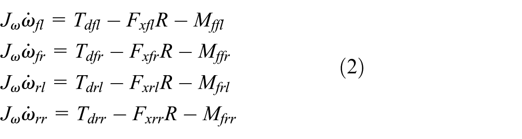
where the subscripts fl, fr, rl, and rr denote the front-left wheel, front-right wheel, rear-left wheel, and rear-right wheel, respectively, and have the same meaning in the following sections.
Vehicle condition parameters estimation
It is more straightforward to estimate the probability density distribution of nonlinear functions than the nonlinear function itself, 13 and thus we designed our vehicle condition parameter estimation using a UKF to approximate a nonlinear function. The core algorithm of UKF is unscented transform (UT), that is, in the original state distribution, the set of points is selected according to certain rules such that the mean and covariance of the set are equal to the mean and covariance of the original state distribution. The point set is then plugged into the nonlinear function to obtain the corresponding value of the nonlinear function. Unlike an EKF estimation method, UKF does not require calculating the Jacobian matrix complex, thus preventing truncation errors owing to the Taylor expansion of the nonlinear system.
The general nonlinear system can be described using a state space equation encompassing the state equation and measurement equation. Its discrete form is as follows

where
The necessary vehicle state parameters defined for observation are as follows

The measurement variables are

The longitudinal tire force can be obtained using the motor torque and equation (2), and
According to the vehicle model, the magic formula tire model 14 and tire vertical force formula comprise the estimator state equation (7), and the measurement equation (8), shown below


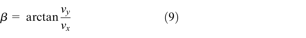
The vehicle sideslip angle is
where B, C, D, and E are the fitting coefficient for the magic tire formula. 15
UKF estimation process
Filter initialization
The nonlinear system has system and measurement noises, and thus the extended vector is defined as

The 2n + 1 Sigma sampling point
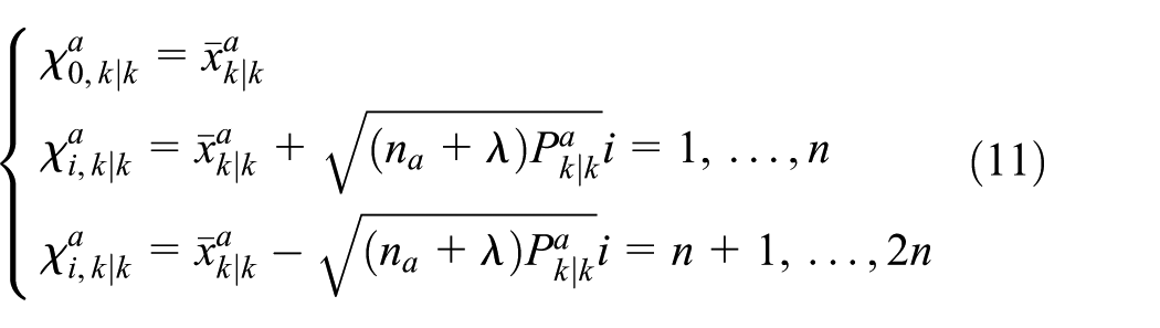
The Sigma point weight
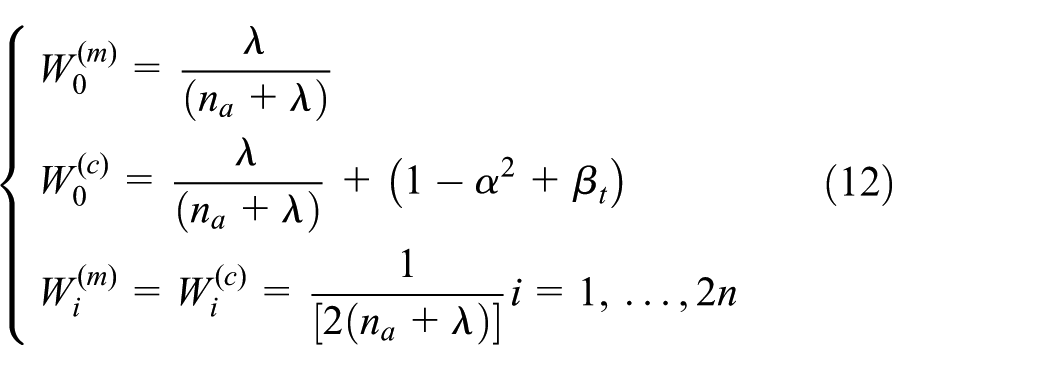
where
UKF calculation
The time update functions

The measurement update functions

Active yaw moment controller
Two degrees of freedom vehicle model
The vehicle model can be considered as having two degrees of freedom (2DOF), namely, lateral motion along the y-axis and yaw motion about the z-axis, when the vehicle is driving at a constant velocity. The following assumptions are made for a vehicle model: (1) The lateral acceleration is below 0.4 g, (2) the lateral characteristics of the tire are within a linear range, (3) the suspension effects are ignored, (4) the aerodynamics are ignored, and (5) under a steady state,


The following equation can be obtained from the vehicle linear 2DOF model shown in Figure 3


2DOF vehicle model.
Considering the state of stability of the vehicle, the steady-state yaw rate gain and steady-state sideslip angle gain are obtained from equation (17).
The steady-state yaw rate gain is as follows
The steady-state sideslip angle gain is the following

where K is a stability factor

Because the 2DOF vehicle model analysis does not include the longitudinal motion of the vehicle, the effects of the longitudinal force on the yaw moment are not reflected in equations (15) and (16); in other words, they only include information about the yaw moment caused by the lateral tire force. However, for certain practical application, the control of the yaw moment is only achieved by controlling the torque of the in-wheel motor, that is, only the longitudinal tire force is controllable. Thus, to remedy this, it is necessary to added the following to equation (16)

where
Active yaw moment controller based on SMC
The sideslip angle and yaw rate are two important state variables that measure the vehicle stability. The goal of the stability control is to keep

where c is the joint control parameter.
According to the exponential reaching law obtained in this the arrival conditions 16

According to the Lyapunov function

and therefore, the system is guaranteed to be stable.
The following equation holds

where k is the coefficient of the defined sliding surface, and
Substituting equation (24) into equation (20) yields the additional yaw moment in which

Torque distribution controller
Objective function
We used the minimum vehicle tire utilization as the objective function. 17 This allowed us to reduce the possibility of sliding or locking the wheel while reasonably allocating the load of each tire, 18 providing a sufficient tire adhesion margin to maintain the level of stability. If the all tire utilization reaches a maximum of 1, the tire meets the limits of adhesion and external influences threaten the vehicle stability.
The tire utilization formula is

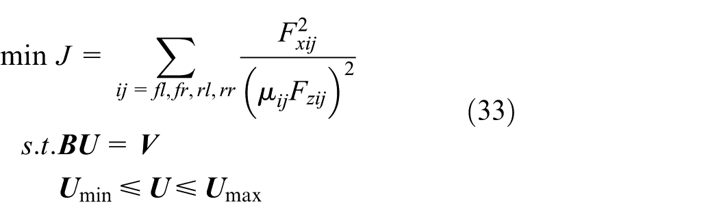
The minimum sum of the four tire utilization squares serves as the objective function. The 4WID electric vehicle has a longitudinal drive force that is independently controllable, whereas the lateral tire force cannot be directly controlled. Therefore, we revised the objective function accordingly to control the longitudinal tire force and minimize its utilization to avoid longitudinal tire force saturation to affect vehicle stability. The objective function obtained after rewriting is as follows

The objective function is expressed in matrix form

where

and

Objective function constraint
The active yaw moment controller is used to calculate the additional yaw moment required to maintain the vehicle stability during transit. The additional yaw moment is achieved by controlling the longitudinal force of the tire, and thus, it is necessary to distribute the wheel torque; the distributed torque must satisfy the driving force of the vehicle. We designed two control inputs for this purpose: the additional yaw moment
The additional yaw moment was calculated via equation (25) and the generalized longitudinal force via PI control. It is necessary to ensure that the actual longitudinal acceleration is close to the driver’s intended acceleration, which is expressed through the following equations

where
When the vehicle is operating, the power and stability are maintained as long as equation (30) is satisfied

Equation (30) also reveals the relationship between the control and output parameters. Therefore, the equality constraint of the objective function can be obtained

where

The torque provided by the drive motor is limited by the maximum torque of the motor. According to the design requirements,

Objective function solution
Nonlinear programming method
The electric vehicle torque distribution problem was solved based on the nonlinear programming (NP). The standard form of the NP is
This problem can be solved by using fmincon tool in a MATLAB optimization toolbox. With this method, the solution method can be autonomously chosen according to the calculation applied, such as a sequence quadratic programming (SQP) algorithm, an interior point penalty function method, or a feasible set method, among others.
Quadratic programming method
According to the above optimization objective function and the constraint condition, the torque distribution problem can be solved via quadratic programming (QP). The standard form of the QP method is

This problem can be solved using the quadprog tool in the MATLAB optimization toolbox.
By comparing equations (33) and (34), the objective function of the NP is similar to the QP. As the difference between the two, the objective function of the NP is not required to form the objective function, whereas QP requires transforming the objective function, for example,
Weighted least squares method
The independent driving electric vehicle torque distribution problem can also be formulated as a weighted least squares (WLS) problem. Equation (34) is the optimal solution to the objective function within the range of equation (30), and thus, the objective function and constraint condition can be transformed into the SQP form

The feasible solution field is
Here,
The SQP solution steps are more cumbersome. First, the feasible solution domain is guaranteed as a precondition for the optimal solution. This degrades the real-time performance of the algorithm. We introduce the weight coefficient

Equation (36) can be transformed into a standard least squares form using the deformation shown in equation (37), which can be solved through the least squares tool in the MATLAB optimization toolbox

Simulation results
To validate the estimation results of the vehicle state estimator, we conducted a double line change (DLC) simulation test under a vehicle speed of 100 km/h and road adhesion coefficient of 0.8. The driver model for the steering wheel angle input was established in CarSim software using a preview time set to 1 s. The vehicle parameters were selected according to CarSim, as shown in Table 1. CarSim is a widely used vehicle simulation program and has high credibility, ensuring the reliability of the simulation test results. 20 The DLC path was set as shown in Figure 4, and the results of the UKF are shown in Figures 5–7.
Simulation parameters of the vehicle.

CG: center of gravity.

DLC test path traffic cones setting.
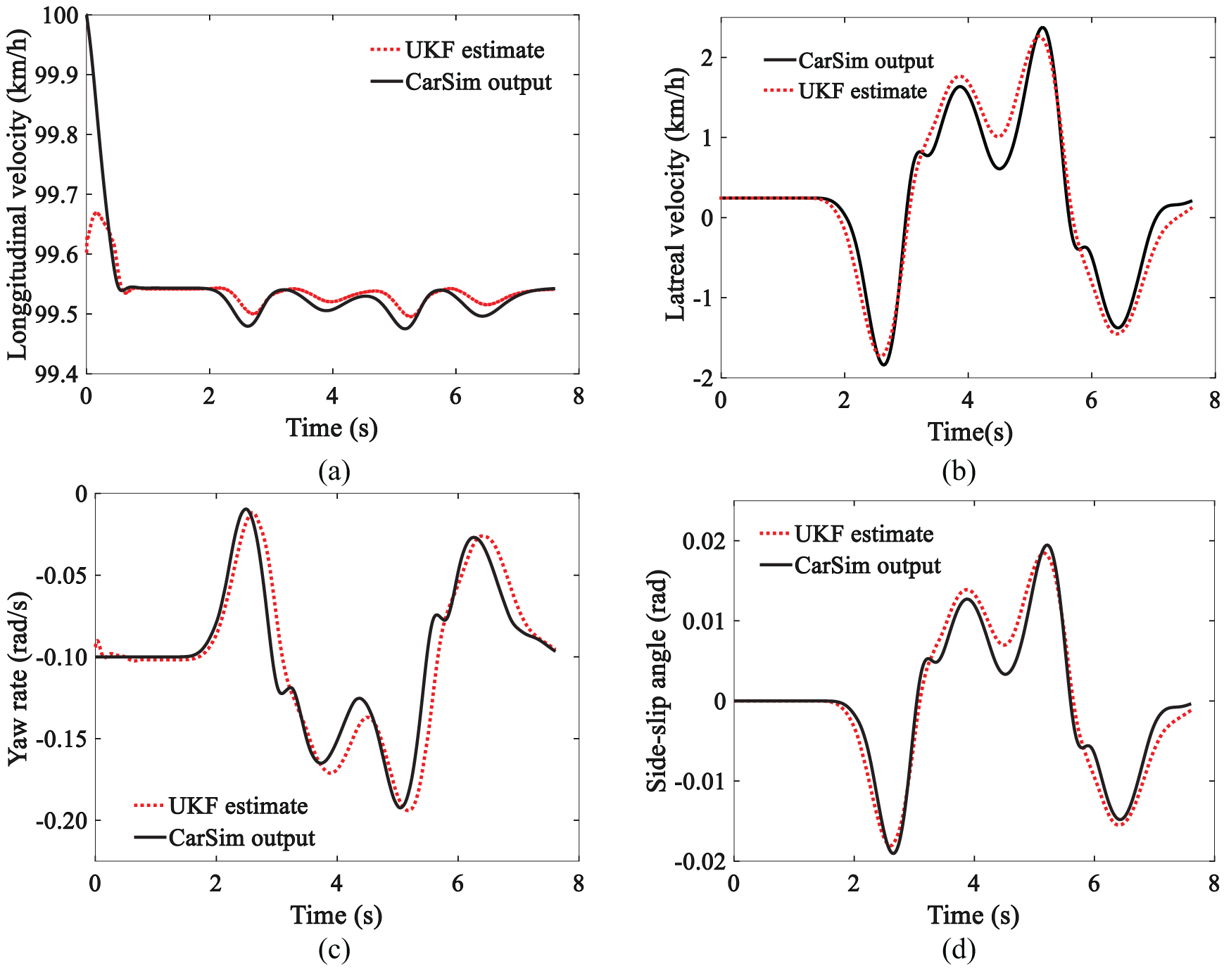
Estimation results of vehicle condition parameter: (a) Vehicle longitudinal velocity, (b) vehicle lateral velocity, (c) Yaw rate and (d) sideslip angle.
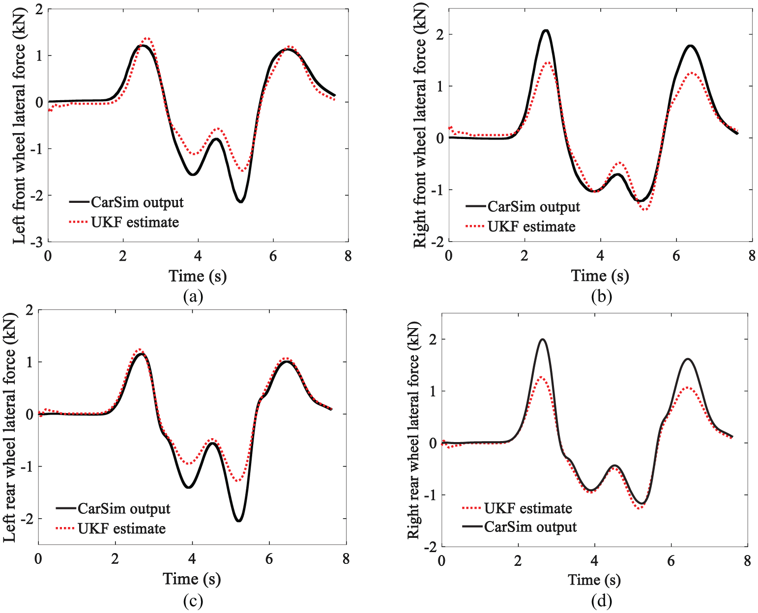
Estimation results of vehicle condition parameter: (a) Left front wheel lateral force, (b) Right front wheel lateral force, (c) Left rear wheel lateral force and (d) Right rear wheel lateral force.

Estimation results of vehicle condition parameter: (a) Left front wheel vertical force, (b) Right front wheel vertical force, (c) Left rear wheel vertical force and (d) Right rear wheel vertical force.
Figure 5(a)–(d) show the vehicle speed, yaw rate, and sideslip angle estimation results of the vehicle state estimator, all of which are accurate. Figure 6(a)–(d) show the lateral tire force estimation results in which an error is shown at the peak, because the tires in this stage of force change violently and are highly nonlinear; the magic formula tire model for fitting the lateral force contains an error under these conditions. Figure 7(a)–(d) show the vertical force estimation results of the tire, where the proposed estimator is again highly accurate.
To verify the control effect of the active yaw moment controller and torque distribution controller, we conducted a DLC simulation test with a vehicle speed of 100 km/h and road adhesion coefficient of 0.4. The DLC path was set as shown in Figure 4. Three methods of torque distribution were tested. The active yaw moment controller output results are shown in Figure 8, the results of three methods of vehicle stability control are shown in Figure 9, and their resulting torque distribution are shown in Figure 10. “Method 1” indicates the NP, “Method 2” represents the QP, and “Method 3” is the WLS.

Additional yaw moment controller outputs.

Three optimization methods for stability control: (a) Control before and after vehicle sideslip angle. (b) Control before and after yaw rate. (c) Control before and after

Three optimization methods torque distribution results: (a) Torque outputs under NP control. (b) Torque outputs under QP control. (c) Torque outputs under WLS control.
Figure 8 shows the output of the active yaw moment controller based on the SMC, which is one of the constraints of the torque distribution controller. Figure 9 shows the control results of the three vehicle drive torque distribution methods tested. We used two important parameters, yaw rate
In the following, we will analyze the characteristics of three methods. As we all know, variance is a useful method to represent data fluctuations. However, the mean of the three methods has a large difference, so it is not advisable to directly compare the variance of the data. Thus, we have adopted another method to represent the fluctuation of data. First is the pairwise combination of the data of three methods, followed by the calculation of the differences of these combinations and, finally, calculation of the variances or means of the above differences. The calculation method is as follows


where
Comparison of three optimization methods.

QP: quadratic programming; NP: nonlinear programming; WLS: weighted least squares.
All three methods perform similarly in providing effective vehicle stability control as shown in Figure 9 and
Run time of three methods.

QP: quadratic programming; NP: nonlinear programming; WLS: weighted least squares.
Conclusion
This article presented a novel vehicle stability controller comprised of a vehicle state estimator, active yaw moment controller, and torque distribution controller. The vehicle state estimator was designed based on a UKF, the active yaw moment controller was designed based on the SMC theory, and the torque distribution controller was based on three mathematical optimization algorithms.
The UKF-based vehicle state estimator was shown to accurately estimate such parameters as the vehicle speed, sideslip angle, yaw rate, and tire force. This lays the foundation for acquisition of the active yaw moment control and torque distribution control information.
We simulated a DLC using a high-speed and low adhesion coefficient under which the proposed controller performed extremely well.
The control output results of the NP, QP algorithm, and WLS method were compared, and it was determined that all three are feasible but with different advantages and disadvantages. The NP and QP showed the best stability, whereas the WLS method showed the fastest calculation time.
In a future work, we will apply hardware-in-the-loop testing on the algorithm to verify the real-time performance of the control method in the C programming language environment.
Footnotes
Appendix 1
Handling Editor: Sunan Huang
Declaration of conflicting interests
The author(s) declared no potential conflicts of interest with respect to the research, authorship, and/or publication of this article.
Funding
The author(s) disclosed receipt of the following financial support for the research, authorship, and/or publication of this article: This work was supported by the Chongqing Research Program of Basic Research and Frontier Technology (cstc2018jcyjAX0109) and by the National Natural Science Foundation of China (51205433).