Sage Journals: Discover world-class research

Abstract

Vibration prediction plays a vital role in the environmental assessment of new railway lines and the vibration analysis of new buildings near railway lines. We use theoretical analysis, numerical simulation, and field experiment, which can help predict vibration with high accuracy. These methods have their own advantages, but are time-consuming or costlier. This article outlines a fast, high-accuracy prediction method combining the advantages of numerical simulation, experiment, and artificial neural network. The method takes artificial neural network as one of the supervised machine learnings, and it is founded upon a fully validated three-dimensional finite element model. First, establish a three-dimensional finite element model using ANSYS software and generate series of samples by changing field conditions. Then, create an artificial neural network and train it by the samples obtained from FEM and experiment. Finally, use the artificial neural network that has been trained to predict the level of vibration on certain conditions. The result states that the predicted method can control the maximum error below 6.41% and the average error below 2.29% when it is used to predict acceleration vibration level. An advantage of this method is that it spends zero time on predicting vibration level. A key benefit from this decreased prediction time is that it potentially reduces the detailed vibration analyses required for a new train line so that it can reduce project costs. In addition, it could also consider the effect of soil parameters.

Keywords

Artificial neural network railway vibration prediction numerical model

Introduction

The Railways has experienced a quick international growth in recent years, especially the high speed railway, and the issue of environmental vibration near train lines has been troubling at the same time. The vibration not only causes significant negative effects, such as personal insomnia and anxiety, but also affects the accuracy of precision instruments. Every new line needs to assess the impact on environment, which includes deciding the level of vibration at the planning stage. Theoretical analysis, numerical analysis, and field experiment are generally used to assess vibration level, but these methods require more time or are of high costs, if we consider detaining. We usually simplify calculation model at the expense of assessment accuracy. This article presents a rapid and high accurate method artificial neural network (ANN) model, founded by detailed three-dimensional finite element model (3D FEM). We could assess vibration level within a certain distance near rail lines through the ANN with high accuracy and zero time line.

Zhai et al.¹ researched on characteristics of ground vibration acceleration in both time and frequency domains through a field measurement on Beijing–Shanghai high-speed railway. Connolly et al.² did experiments on various earthwork profiles and analyzed experimental data. It is found that horizontal vibrations should be considered, and embankment earthwork profiles produced the lowest vibration levels and the cutting produced the highest vibration levels. And he also did some experiences to quantify the level of error that can be expected in the literature.³

Shih et al.⁴ presented an investigation using finite element models in time domain to present a load moving on a railway track on a flexible ground. A systematic study is carried out to compare different sizes and shapes of finite element mesh with different boundary conditions. He developed finite and infinite element models, and compared the results. The compared result showed that the finite element model can meet the accuracy requirements, and it is more suitable to use finite element modeling considering various factors.

Yao et al.⁵ developed a model that is used to predict vibration of building based on support vector machine (SVM) and wavelet analysis. This article analyzes in detail the effects of different factors on building vibration caused by trains. This article also analyzes the data obtained from the experiment based on wave theory, selects samples to train the SVM prediction model, and then uses the trained model to predict the vibration of the building and to compare it with the field test data. The results show that this method can achieve higher prediction accuracy.

Paneiro et al.⁶ predict ground vibration amplitude on buildings through ANN, and quantitative field data about ground vibration can be obtained through railway traffic in urban areas. They used those data only to train ANN. Limitations of using only field quantitative of the vibration propagation media were overcome by including qualitative data available about the propagation media. The limitation of this article is that it does not consider detailed properties of soil and soil parameters separately.

Connolly et al.⁷ developed a new tool to predict vibration that is founded upon using a fully validated 3D FEM to generate synthetic vibration records for a wide range of soil types. Based on this database, the relationships of input and output could be demonstrated through artificial multilayer perceptron neural network architecture. They simplified the secondary suspension into a spring when force of wheel and rail was simulated.

Although numerical analysis method could predict vibration with high accuracy, complex model, long calculation time, and inconvenience in practical application were its drawbacks. ANN based on field test data could reduce the time of calculation and avoid developing numerical model, but it needs a large number of field tests. In addition, the key limitation of this method is that it cannot consider soil parameters.

This article is organized as follows. In “The numerical analysis” section, a FORTRAN program and a 3D finite element mode are developed to simulate wheel–rail contact and site conditions. Combining the two simulation methods we could get each point vibration caused by the moving train. In the same section, the numerical simulation method is compared with the literature⁸ to determine its validation. In “The analysis of each main factors of the site vibration” section, the influence of some main factors, such as distance from railway, soil properties, train speed, and train axle weight, is analyzed. In “Machine-learning approach” section, an ANN model is developed based on the data generated from numerical simulation and experiment. The predicted result is shown in same section. Finally, the conclusion and discussion are provided in the “Conclusion” section. The method process is outlined in Figure 1.

Figure 1.

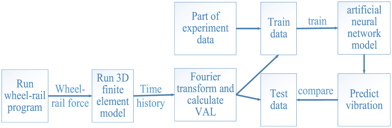
The method process.

The numerical analysis

The ANN model is developed using statistical approach, which is similar to the previous literature works.^8–11 A key difference is that this model is based on the data of high accuracy numerical model and is part of field test data. Thus, soil properties can be obtained when FEMs are developed, and this article considers the effect of soil properties that is hard to achieve using the field site test method because of limitations on site. In addition, this method can be used to analyze the effect of different layers of soil for wave propagation without field test.

The numerical model consists of the train–track–foundation system and FEM of soil. First, wheel–rail forces with different speeds and different axle weights are calculated through wheel–rail forces calculation program developed by Fortran. Force to finite element model is added to calculate site vibration.

The 3D FEM is used in the analysis of the main factors of the site vibration and produced the ANN training data.

The train–track–foundation system

This train–track–foundation system consists of a vehicle model and track model. The train model and the track model are linked through nonlinear Hertzian contact spring between the wheels and the track.¹²

The vehicle model

The vehicle model consists of a locomotive and three same trailers, and each of them is modeled using a lumped mass multibody approach including car, bogie, wheelset, secondary spring, and damper, as shown in Figure 2. The car, bogies, and wheels are connected using springs and dash-pots to model the vehicle suspension characteristics. Each wheel is coupled with the rail using a nonlinear Hertzian contact spring.

Figure 2.

The calculation diagram of the vehicle model.

Each car or bogie considers two freedoms including nodding and floating, whereas each wheel considers only floating freedom. A locomotive consists of 10 degrees of freedoms totally.

The main parameters of the vehicle are shown in Table 1.

Table 1.

Main parameters of train vehicles.

Name	Unit	Locomotive	Trailer
Car body quality, M_c	kg	31,600	3050
Bogie quality, M_t	kg	3200	2600
Wheelset quality, M_w	kg	2000	1910
Car body nodding moment of inertia, J_c	kg m²	1.867 × 10⁶	1.279 × 10⁶
Bogie nodding moment of inertia, J_t	kg m²	1.753 × 10³	1.424 × 10³
First suspension stiffness K_pz (each axis)	N/m²	2.352 × 10⁶	2.488 × 10⁶
Secondary suspension stiffness, C_pz (each axis)	N s/m	1.96 × 10⁵	3.92 × 10⁵
Secondary suspension stiffness, K_sz	N/m	2.2291 × 10⁶	1.982 × 10⁶
Secondary suspension damping, C_sz	N s/m	1.174 × 10⁶	1.96 × 10⁶
Vehicle length, l	m	25	25
Vehicle distance, l_c	m	17.5	17.5
Bogie wheelbase, l_t	m	2.5	2.5
Wheel radius, R	m	0.43	0.43

This article establishes the motion equation of locomotives using Lagrange equation, which is showed as follows

\frac{d}{dt} (\frac{\partial T}{\partial {\overset{\cdot}{q}}_{k}}) - \frac{\partial T}{\partial q_{k}} + \frac{\partial V}{\partial q_{k}} + \frac{\partial Q}{\partial {\overset{\cdot}{q}}_{k}} = 0

(1)

Where T, V, Q are total kinetic energy, total elastic potential energy, and total damper dissipation energy of the motion system, respectively.

The motion system of body, bogie, and wheelset can be established based on the Lagrange motion equation.

The motion equation of the ith body and its two bogies is as follows

M_{i} {\overset{\cdot\cdot}{Z}}_{i} + C_{i} {\overset{\cdot}{Z}}_{i} + K_{i} Z_{i} = P_{i} (t), i = 1, 2, \cdot \cdot \cdot, N_{v}

(2)

Where Z_i is the displacement vector of the ith vehicle; P_i(t) is the external excitation force for the ith vehicle, and M_i, C_i, and K_i show the mass, damping, and stiffness of the ith vehicle model, respectively.

The track model

The track is in the form of ballast, consisting of rails, sleepers, roadbed, and subgrade, and it is simulated as a three-layer discrete model. Rails are regarded as Euler beams supported by discrete points. Foundation is divided into discrete element on basis of sleeper support points. Every element consists of two messes and three layers of spring-damping. Adjacent elements are connected by shear spring-damping. The model is shown in Figure 3.

Figure 3.

The calculation diagram of the track mode.

The wheelset connects with the track in accordance with Hertz wheel–rail contact relationship. The vibration in the vertical longitudinal plane of the model is only considered. It is due to the fact that the vertical excitation for the bottom roadbed caused by the locomotive axle load of the moving train is much larger than the horizontal excitation.

Three-dimensional finite element model

To simulate the vibration site and analysis of each main factors of the site vibration, a 3D FEM is developed using finite element software ANSYS. The model consists of rail, sleeper, ballast, and subgrade.

The track is modeled according to the literature,¹³ and the result of this model is compared with the literature¹³ to prove the model validation. This model is simplified to reduce calculate time. In order to simulate the whole process of a train entering and leaving the site and considering the phase difference of each load the length along the track is 148.5 m. To reduce the effect of the reflection of the wave at the boundary on the vibration, to observe the vibration in a wide range as much as possible, and also considering the calculation time, the width of the vertical track is 120 m. The depth in vertical track is 47.8 m, which has two layers, as the soil layer with detailed parameters is 47.8 m. The model includes 1,02,06,932 nodes and 2,69,481 elements. The size of the model is shown in Figure 4.

Figure 4.

Three-dimensional finite.

The rail is supported by concrete sleepers laid each at a distance of 0.55 m. Sleepers are then supported by ballast that is modeled with the subgrade in this article. The contact between rail, sleepers, and ballast are not considered for rail fasteners.

Ballast, subgrade, and site are simulated by solid45 element. The right and lower extents of the boundary use 3D viscoelastic-damping elements to simulate absorbing boundary condition that could prevent the reflection of waves.¹⁴ The boundary of front and back are considered as free surface. The boundary of left uses symmetrical boundary.

Many physical soil profiles consist of many layers, but to reduce calculation conditions and calculation time the numerical model considers only two layers of soil. Multilayer soil is translated to two layers of soil using weighted average.¹⁵ The translation formula is shown as follows

E_{eq} = \frac{\sum H_{i} E_{i}}{\sum H_{i}}

(3)

Model validation

This article using the data from 3D FEM compares with test data in the literature¹³ to determine whether the prediction data could satisfy sufficient accuracy by this model. This experiment was completed by the author’s research group.

The Figure 5 is the compared result between measured values and calculated values. The result shows that calculated value fits well to measured values. The maximum error is 7.5% and the average error is 2.9%. The results show that the 3D FEM can effectively simulate the situation on site.

Figure 5.

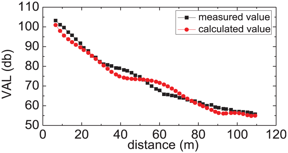
Comparison of measured and calculated data.

Field work

The experiment was carried out in a playground near the Beijing–Guangzhou line, and there is no building around the playground. The parameters of the site soil are shown in Table 2. The thickness of the bottom layer soil is artificially increased 30 m, in order to reduce the influence of the boundary conditions at the bottom edge and other parameters are consistent with literature.¹³ The train speeds range from 21 km/h to 128 km/h, and train type contains freight train and passenger train. In this article, the data of a passenger train with speed of 67 km/h and weight of 160 kN is compared to ensure that the numerical model and the ANN can predict vibration with high accuracy.

Table 2.

Soil properties in experimental site.

Soil layer	Thickness, m	Bearing capacity, kPa	Compression modulus, Mpa	Moisture content, (%)	Density, (g/cm³)
Silty clay	0.5–2.0	150	17.0	19.6	1.91
silt	2.0–2.4	130	17.5	24.0	1.82
Silty clay	2.0–2.3	150	17.5	21.2	1.75
silt	2.2–3.0	160	18.5	22.1	1.90
Fine sand	1.9–2.5	200	18.0	22.5	1.95
Coarse sand	5.4–5.6	320	22.0	22.0	2.11
silt	2.8–30.0	150	16.5	23.6	1.90

Data processing method

The data of the field and numerical simulation is acceleration. We need to change the data to frequency domain using Fourier transform and analyze each center frequency of one-third octave. Then, the ground surface vertical VAL can be obtained according to ISO2631 developed by the International Organization for Standardization. VAL is calculated by the following formula

L_{a} = 20 \times \log_{10} (\frac{a}{a_{ref}})

(4)

Where L_a/dB is the VAL; a_ref is the reference vibration acceleration, valuing 1 × 10⁻⁶; a (m/s²) is the vibration acceleration root mean square (RMS) shown as follows

a = \sqrt{\sum a_{f_{rms}}^{2} \cdot 10^{0.1 c_{f}}}

(5)

where a_f_rms (m/s²) is the acceleration RMS at frequency f; c_f is the sensory correction of the acceleration vibration corresponding to different frequencies.

The analysis of each main factors of the site vibration

During analysis, one parameter is changed and other parameter remains constant. The value of each parameter is shown in Table 3 except for special declaration.

Table 3.

Parameters of numerical model.

Train type	Speed	Train axleweight	Damping ratio(two layers)	Elastic modulus(Soil Layer 1)	Elastic modulus(Soil Layer 2)	Density(Soil Layer 1)	Density(Soil Layer 2)
CRH2	67 km/h	160 kN	0.005	17.7 Mpa	16.9 Mpa	1.83 g/cm³	2.02 g/cm³

The influence of the soil properties

When analyzing the characteristics of soil, the multilayered soil is simplified into two layers, and the parameters of the two layers of soil change at the same rule.

The influence of damping ratio

The damping ratios of the two layers of soil have the same range values, which are 0.05, 0.1, 0.15, 0.2, 0.25, respectively. The vertical acceleration of each measurement point is converted to VAL for analysis. The result is shown in Figure 6.

Figure 6.

The vibration caused by different damping ratios.

Through calculation results, the following conclusions are obtained.

As the damping ratio increases, the VAL of each point becomes smaller, especially when the damping ratio increases from 0.05 to 0.1, and this difference becomes smaller when the damping is greater than 0.1.

As the damping ratio increases, the attenuation of the vibration becomes faster. The farther away from the center of the orbit, the greater the difference between the VALs at the same point with different damping ratios.

The influence of elastic modulus

It is difficult to use the same value for analysis due to large difference between the soil layers.

Therefore, the elastic modulus of the two layers of soil changes by the same multiple, which are 0.1 times, 1 times (the parameters are same as Table 2), 10 times, 20 times, 30 times, respectively.

According to Figure 7, it can be attained that

The vibration decays slowly as the distance increases, when the elastic modulus increases.

When the elastic modulus increases, the vibration at a point closer to the orbit becomes smaller, and the vibration at a point farther from the orbit becomes larger.

When the elastic modulus is less than a certain value, the vibration becomes volatility attenuation as the distance increases.

Figure 7.

The vibration caused by different elastic modulus.

The influence of density

Similar to elastic modulus, the density of soil also changes by the same multiple which are 0.75 times, 1 times (the parameters are same as Table 2), 1.25 times, 1.5 times, 1.75 times. The result is shown in Figure 8.

Figure 8.

The vibration caused by different densities.

According to the calculation result, it can be attained that

The VAL of each point produced by the moving train becomes gradually smaller with the increasing density.

As the distance from the center of the track increases, the VAL difference becomes larger at each point of different densities, especially within 40 m from the center of the track.

The influence of Poisson’s ratio

Figure 9 reflects that the Poisson ratio varies from 0.2 to 0.4 and has little effect on the VAL. When the distance from point to the center of the track is within 80 m, the vibration level decreases with the increase of the Poisson’s ratio for the same point. However, when the distance from the measuring point to the track is greater than 80 m, this phenomenon is just the opposite.

Figure 9.

The vibration caused by different Poisson’s ratios.

Parameter sensitive analysis

It could improve prediction accuracy if all soil properties be considered when predicting vibration by ANN. Each property needs to be expressed by a parameter. Thus, the number of calculated conditions will increase exponentially and calculation time becomes unacceptable. Therefore, it is necessary to reduce calculation parameters. This article considers only two soil properties that have the least influential on vibration.

In the analysis of soil parameters sensitivity, the finite element model is same as above, except the soil parameters of the two layers soil (does not include roadbed). The points of calculation lie in the surface of the middle section of the FEM.

The value of each parameter to be analyzed increases by 15%, which includes damping ratio, Poisson’s ratio, elastic modulus, density, and other parameters remain constant. Wheel and rail forces were loaded onto 3D FEM to obtain time-course data. Then VAL levels are calculated using the results of the previous step. The VAL value of each point with different property is compared with the result of them before unchanging the parameter. The results can be seen in Figure 10. It can be seen from the analysis results that damping ratio has the greatest impact on the results, followed by density. Therefore, damping and density have a greater impact on vibration at the same ratio.

Figure 10.

The comparison of different soil properties.

However, usually the range of different parameter variations is large, so the range of variation of parameters must be considered. Then, calculate the relative vibration difference between each parameter and the contrast value under different parameters, and then multiply the relative vibration difference by the coefficient of variation of the parameter. The formula is as follows

Δ VAL = (VA L_{i} - VAL') • ξ_{i}

(6)

ξ_{i} = \frac{x_{\max} - x_{\min}}{x_{\min}}

(7)

where VAL_i represents the acceleration vibration level of different parameters; VAL’ is the acceleration vibration level without changing any parameters. X_max and X_min are the maximum and minimum values of different parameter variation ranges. ζ_i is coefficient of variation of the parameter.

It can be seen from Figure 11 that when considering the variation range of these parameters, elastic modulus and damping ratio have a greater influence than other factors on the vibration, so elastic and damping ratio are selected to represent the characteristics of soil.

Figure 11.

The comparison of different soil properties (considering the variation range of the parameters).

The influence of the train speed

This article analyzes five train speeds, which are 33 km/h, 67 km/h, 100 km/h, 134 km/h, and 167 km/h. Figure 12 shows the changing curves of points at different distances from the track.

Figure 12.

The vibration caused by different train speeds.

From Figure 11, it can be attained that when the speed is 33 km/h, the VAL of each point is the largest. When the speed is 134 km/h, the VAL of each point is the smallest. When the speed reaches a certain value, the vibration becomes volatility attenuation, which is most obvious at a speed of 134 km/h. However, when the speed is 167 km/h, this phenomenon is weakened.

The influence of different train axle weight

The train has five kinds of axle weight, which are 122 kN, 128 kN, 144 kN, 160 kN, 176 kN, respectively. The impact is analyzed among different axle weight at the speed of 67 km/h. The result is shown in Figure 12.

According to Figure 13, it can be attained that the axle weight has little effect on the VAL within 40 m from the center of the track. When the distance from the point to the track is greater than 40 m, the VAL decreases with the increase of the axle weight. It is obvious when the axle weight is 176 kN. As for other axle weights are considered, it is obvious after 80 m from the track. The reason is that as the axle weight increases, the high-frequency component of the vibration increases, and the low-frequency component decreases. During the propagation of the wave, the high-frequency component attenuates faster due to the filtering effect of the soil, and the low-frequency component attenuates slowly. Therefore, the larger the axle weight, the smaller the VAL.

Figure 13.

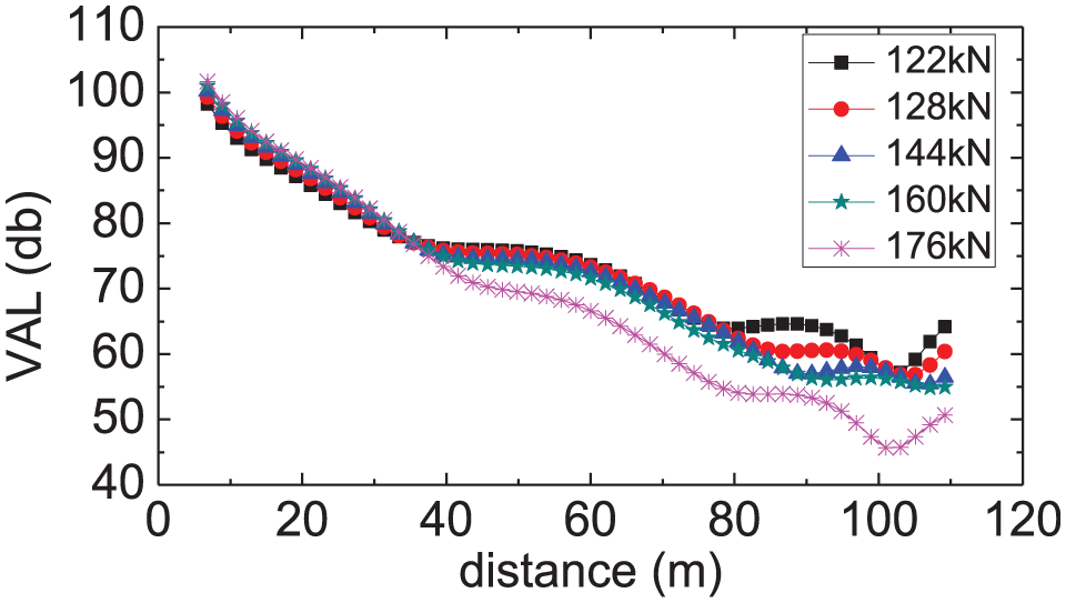
The vibration caused by different train axle weights.

Machine-learning approach

An ANN approach is used in this article to predict vibration because of its nonlinear regression capability. Wave propagation is a major factor affecting site vibration; therefore, the accuracy of wave propagation prediction will directly affect the accuracy of vibration prediction. ANN model has been used successfully in wave propagation modeling to predict the propagation of bomb blast wave,^16,17 to predict ground vibrations induced by impact driving of piles,¹⁸ to analyze dynamic response of multilayered ground under moving loads of various distributions,¹⁹ and to predict the building response due to ground vibration.²⁰

An error back-propagation (BP) training algorithm is used in ANN to map the inputs and outputs. ANN has an input layer, an output layer, and many hidden layers. Algorithms can be used to map input layer data to output layer data. BP algorithm can feedback errors through the network. First of all, the training patterns are propagated forward through the network and compare with the output targets. The error between output and target then propagate back through the network and the weights are updated. The next train is based on the latest weight until the last train, and the model has the minimum error. The ANN model is shown in Figure 14.

Figure 14.

Artificial neural network.

To obtain data for training and comparing, the ANSYS model is computed for 625 permutations of input parameters, and 37,500 data points are used in the network.

Each time the numerical simulation will generate a time history. The frequency spectrums and VAL are calculated, which are typically used for analyzing the effect of vibration on human. The metric is used as input data to train the network respectively.^21–23

The instance verification

To ensure that the ANN can predict vibration level with high accuracy at variety of test sites, it is validated using experimental results.

ANN needs to be trained with massive data before being used to predict VAL. The data are obtained using numerical models with 625 working conditions and part of experiment data. The ANN considers train speed, elastic modulus of two layers of soil, train axle weight, and distance from the measuring point to the center of the track. From these data samples, 10% of the simulated data and the field measured data are randomly selected as verification samples, and other data are used as training samples. Training samples are standardized before being entered into the program. After the ANN is trained, the verification accuracy is verified sing the verification samples. The output data of the ANN are subjected to denormalization processing in order to compare with the time history curve of the sample.

Comparison of predicted measured results

One of the working conditions is selected to compare experimental result, numerical calculation result, and ANN prediction result. The working condition is that the train speed is 67 km/h, the train axle weight is 160 kN, the elastic modulus of the upper layer soil is 17.7 Mpa, the elastic modulus of the subsoil is 16.9 Mpa. The compared result is shown in Figure 15.

Figure 15.

Comparison of measured value, calculated value, and predictive value.

According to Figure 15, it can be obtained that

The predicted value obtained by the ANN method has little error with the analog value obtained by the numerical simulation method, and the maximum error value is 2.35%, and the average error value is 0.72%.

The maximum error of the predicted value obtained by the ANN method is 6.41% and the average error is 2.29%, which is 1.19% and 0.58% lower than the numerical simulation method. The result indicates that the predicted model can objectively reflect the propagation rules in the soil.

Conclusion

A network is developed capable of predicting VAL with high accuracy. A 3D FEM is used as an aid to generate training samples. Through the analysis of the soil parameters, it can be seen that the elastic modulus has a greater impact on the vibration. The predicted result shows that it could provide effective data when predicting VAL. This method can be used as an effective means for vibration prediction.

The method of predicting vibration needs zero run time and can consider the elastic modulus of two soil layers. It can predict vibration for built lines in a short time in the early design stage. Furthermore, it can also provide reference for the validity of the 3D finite element calculation model in later detailed analysis.

Footnotes

Handling Editor: Tao Feng

Declaration of conflicting interests

The author(s) declared no potential conflicts of interest with respect to the research, authorship, and/or publication of this article.

Funding

The author(s) disclosed receipt of the following financial support for the research, authorship, and/or publication of this article: This research is financed by the Basic Research Funds of Beijing Jiaotong University through project C17JB00440, C17JB00300 and 2017YJS122.

ORCID iD

Jinbao Yao

References

Zhai

Wei

Song

et al . Experimental investigation into ground vibrations induced by very high speed trains on a non-ballasted track. Soil Dyn Earthq Eng 2015; 72: 24–36.

Connolly

Kouroussis

Woodward

et al . Field testing and analysis of high speed rail vibrations. Soil Dyn Earthq Eng 2014; 67: 102–118.

Connolly

Costa

Kouroussis

et al . Large scale international testing of railway ground vibrations across Europe. Soil Dyn Earthq Eng 2015; 71: 1–12.

Shih

Thompson

Zervos

The effect of boundary conditions, model size and damping models in the finite element modelling of a moving load on a track/ground system. Soil Dyn Earthq Eng 2016; 89: 12–27.

Yao

Xia

Zhang

et al . Prediction on building vibration induced by moving train based on support vector machine and wavelet analysis. J Mech Technol 2014; 28: 2065–2074.

Paneiro

Duião

Costa e

Silva M

et al . Artificial neural network model for ground vibration amplitudes prediction due to light railway traffic in urban areas. Neural Comput Appl 2018; 29: 1045–1057.

Connolly

Kouroussis

Giannopoulos

et al . Assessment of railway vibrations using an efficient scoping model. Soil Dyn Earthq Eng 2014; 58: 37–47.

Yao

Chen

Cao

et al . Short-term traffic speed prediction for an urban corridor. Comput-Aided Civ Inf 2017; 32: 154–169.

Paneiro

Durão

Silva

MCE

et al . Prediction of ground vibration amplitudes due to urban railway traffic using quantitative and qualitative field data. Transport Res D: Tr E 2015; 40: 1–13.

10.

Wang

Shan

et al . Prediction of bus travel time using random forests based on near neighbors. Comput-Aided Civ Inf 2018; 33: 333–350.

11.

Lam

WHK

Tam

ML.

Bus arrival time prediction at bus stop with multiple routes. Transport Res C: Emer 2011; 19: 1157–1170.

12.

Nan

. Vehicle–structure dynamic interaction. Beijing, China: Science Press, 2005, p.10–15.

13.

Chen

et al . Research on the law of surrounding ground vibration cassed by running trains. Eng Mech 2010; 27: 98–103.

14.

Liu

et al . 3D viscous-spring artificial boundary in time domain. Earthq Eng Eng Vib 2006; 5: 93–102.

15.

Brahma

Mukherjee

. A realistic way to obtain equivalent Young’s modulus of layered soil. In: Indian geotechnical conference, 16–18 December 2010, pp.305–308, https://gndec.ac.in/∼igs/ldh/conf/2010/articles/075.pdf

16.

Flood

Bewick

Dinan

et al . Modeling blast wave propagation using artificial neural network methods. Adv Eng Inform 2009; 23: 418–423.

17.

Taheri

Hasanipanah

Golzar

et al . A hybrid artificial bee colony algorithm-artificial neural network for forecasting the blast-produced ground vibration. Eng Comput 2017; 33: 689–700.

18.

Mihalache

Prediction of ground vibrations induced by impact driving of dolphin piles in Caland Canal. Master’s Thesis, Delft University of Technology, Delft, 2016.

19.

Lefeuve-Mesgouez

Mesgouez

Three-dimensional dynamic response of a porous multilayered ground under moving loads of various distributions. Adv Eng Softw 2012; 46: 75–84.

20.

Auersch

Building response due to ground vibration—simple prediction model based on experience with detailed models and measurements. Int J Acoust Vib 2010; 15: 101–112.

21.

Bin

Wenxuan

Zhen

et al . A heuristic algorithm based on leaf photosynthate transport. Simulation 2018; 94: 593–607.

22.

Wang

Song

et al . Optimizing subordinate net points layout of express enterprise with SCE-UA algorithm. P I Civil Eng: Transp. Epub ahead of print 3 March 2018. DOI: 10.1680/jtran.16.00092.

23.

Zhang

Wang

et al . Study on self-tuning tyre friction control for developing main-servo loop integrated chassis control system. IEEE Access 2017; 5: 6649–6660.

Prediction on soil-ground vibration induced by high-speed moving train based on artificial neural network model

Abstract

Keywords

Introduction

The numerical analysis

The train–track–foundation system

The vehicle model

The track model

Three-dimensional finite element model

Model validation

Field work

Data processing method

The analysis of each main factors of the site vibration

The influence of the soil properties

The influence of damping ratio

The influence of elastic modulus

The influence of density

The influence of Poisson’s ratio

Parameter sensitive analysis

The influence of the train speed

The influence of different train axle weight

Machine-learning approach

The instance verification

Comparison of predicted measured results

Conclusion

Footnotes

Declaration of conflicting interests

Funding

ORCID iD

References