Dynamic surface control–based adaptive neural tracking for full-state constrained omnidirectional mobile robots

Abstract

This article studies the neural network–based adaptive dynamic surface control for trajectory tracking of full-state constrained omnidirectional mobile robots. The barrier Lyapunov function method is adopted to handle the full-state constraints of the omnidirectional mobile robot, and thus state variables will never violate the restrictions. Then, the neural network is used to approximate the uncertain system dynamics, and the adaptive law is proposed to adjust the weights. Moreover, the dynamic surface control is adopted to avoid the derivation of virtual variables, and the complexity of the controller can be simplified in comparison with the classical backstepping technique. The auxiliary system is proposed as the compensator to address the input saturation of omnidirectional mobile robots. All signals including tracking errors, state variables, adaptive parameters, and control inputs in the closed-loop system are proved to be uniformly bounded, while the control gains are chosen properly. Numerical simulations are tested to validate the effectiveness and advancements of the given control strategy.

Introduction

Since the omnidirectional mobile robots (OMRs) can move in any direction without reorientation, they have many potential applications in industrial and military area, such as logistics transportation, factory automation, military affairs, and environmental exploration. The modeling and control designs for OMRs are well discussed.^1–6 For example, Conceicao et al. ⁷ considered the modeling and parameter estimation problems for OMRs; Indiveri ⁸ studied the kinematics analysis and control of Swedish wheeled OMRs; Hashemi et al. ⁹ investigated the proportional–integral (PI) control scheme of four-wheeled OMRs; a near-optimal control strategy for a kind of three-wheeled OMR platform was proposed in Kalmar-Nagy et al.’s ¹⁰ work. However, due to the ideal assumptions for system dynamics and working environment, the uncertainties of the model dynamics and the disturbances are not considered in the above references.

In practical applications, the system uncertainties and the disturbances are important aspects for OMRs to realize the high-precision trajectory tracking and should not be ignored when the controller is designed and implemented.^11,12 A new result about robust control by considering decoupling performance for mobile robots with noise and disturbance was first obtained. ¹³ To attenuate the influences of system uncertainties and disturbances, the adaptive technique is a valid scheme. A fuzzy-based adaptive sliding mode tracking control law was presented in Liu and Hsiao’s ¹⁴ work. Considering the unknown bounded uncertainties, Alakshendra and Chiddarwar ¹⁵ suggested a higher-order sliding mode–based adaptive control scheme to study the trajectory tracking of OMRs, and an adaptive law was used to estimate the upper bounds of uncertainties. For the OMRs with structured and unstructured uncertainties, a smooth adaptive sliding mode–based control law was designed, which can improve the tracking performances and avoid input singularity. ¹⁶ An adaptive scheme that could be adopted to tolerate parameter variations and multiple-output delay in the plants was first proposed in Jia’s ¹⁷ work. Xu et al. ¹⁸ applied a neural network (NN)-based adaptive sliding mode control method to study the tracking control problem of OMRs. Ge and Wang ¹⁹ proposed an adaptive NN control scheme for multiple-input multiple-output (MIMO) nonlinear systems. However, the output or state constraints of OMRs are not considered in these studies. In practical applications, the constraints exist ubiquitously in various aspects which are caused by mechanical structures, actuator saturation, and safety requirements. ²⁰

For the state-constrained single-input single-output (SISO) nonlinear systems, an adaptive output feedback control law was considered. ²¹ The barrier Lyapunov function (BLF)-based adaptive NN control was given for direct current (DC) motor systems. ²² An adaptive NN-based control approach for wheeled mobile robots with full-state constraints was proposed. ²³ Jiang et al. ²⁴ proposed a cerebellar model articulation controller (CMAC)-based NN control strategy with the BLF method to achieve the state-constrained tracking performance. But the above proposed methods are all dependent on the conventional backstepping technique. Note that the classical backstepping approach needs to repeat computing the differentiation of nonlinear virtual signal in each step of backstepping, which can result in the explosion of complexity problem when the system’s order increases. ²⁵ The undesirable numerical noise and heavy computational burden can be caused by these complicated algorithms in practical applications. Dynamic surface control (DSC)^26–29 was also a backstepping-based approach, but it can overcome the explosion of complexity problem by applying the low-pass filters at each step of the backstepping procedure. The transient performance was ensured by the predictor-based neural DSC to avoid the high-frequency oscillation. ²⁹ The controller can also be designed with these low-pass filters when the model cannot be differentiated. Furthermore, in the practical mechanical systems, the control inputs are limited by the capacity of actuators, and the tracking performance of the closed-loop system will be degraded if the input constraints are not considered. Moreover, inaccuracy, instability, and safety accidents may be caused by input limits. In Wen et al.’s ³⁰ work, two robust adaptive control schemes were proposed, where the Nussbaum function was adopted to deal with the nonlinear term caused by the input saturation. The anti-saturation adaptive control approach for MIMO systems based on command filter is analyzed by designing an auxiliary system to compensate for the influence of input constraints. ³¹ Chen et al. ³² proposed a control method of designing time-varying feedback parameters based on the vector decomposition for the mobile robot with diamond-shaped input limits. The novel command governor scheme was introduced to optimize the control input signals in the restricted area, which transformed the state and input constraints to a quadratically constrained optimization problem,^33,34 and in comparison with the traditional model predictive control method such as Liu et al.’s ³⁵ work, better tracking performance can be achieved with Peng’s control strategy. Accordingly, to our best knowledge, the result about NN-based adaptive DSC control of full-state constrained OMRs subject to input saturation has not been published yet.

Based on the above discussions, a novel NN-based adaptive DSC approach will be proposed to solve the trajectory tracking of full-state constrained OMR with system uncertainties and disturbances. The NN-based adaptive technique is employed to approximate system nonlinear dynamics. The DSC is combined with the BLF to design control law to guarantee that all the signals in the OMR system are uniformly bounded and the full-state constraints are not violated. To advance knowledge in this area, this article makes the following contributions:

1. Compared with the trajectory tracking control schemes of OMRs,^14–16,18 the state constraints for position, rotation angle, longitudinal velocity, transverse velocity, and rotating speed are considered in this article, which can guarantee the safety or meet requirements of the operating environment in practical applications.

2. Compared with the backstepping-based control schemes of full-state constrained nonlinear systems,^21–24 the NN-based adaptive DSC control approach is proposed. Because the second-order filter is used at each step of the backstepping procedure, the explosion of complexity problem can be eliminated. Moreover, the input saturation is handled with the anti-windup compensator, which can further ensure the tracking performance.

The rest of the article is divided as follows. Section “System description and problem statement” introduces the kinematic and dynamic model of a class of three-wheeled OMR with model uncertainties. Section “Controller design” gives the implementation process of the control strategy. Numerical simulation results are shown in section “Numerical results” to verify the advantages of the proposed method. Finally, in section “Conclusion,” the entire article is summarized with conclusions.

System description and problem statement

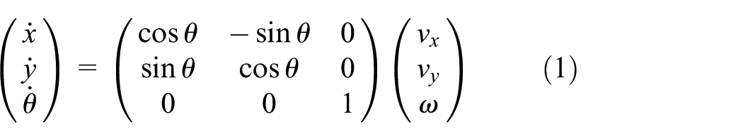
Consider the kinematics and dynamics of a kind of three-wheeled OMR, ¹ and the kinematic model can be given as follows

$$\left(\begin{array}{c}\stackrel{·}{x}\hfill \\ \multicolumn{1}{c}{\stackrel{·}{y}}\\ \multicolumn{1}{c}{\stackrel{·}{\theta }}\end{array}\right)=\left(\begin{array}{ccc}\cos \theta \hfill & -\sin \theta \hfill & 0\hfill \\ \multicolumn{1}{c}{\sin \theta }& \cos \theta \hfill & 0\hfill \\ \multicolumn{1}{c}{0}& 0\hfill & 1\hfill \end{array}\right)\left(\begin{array}{c}{v}_x\hfill \\ \multicolumn{1}{c}{v_y}\\ \multicolumn{1}{c}{\omega }\end{array}\right)$$

(1)

where $(x,y,\theta {)}^{\mathrm{T}}$ represent the position and rotation angle in the world coordinate system, respectively; $(v_x,v_y)$ denote the longitudinal velocity and transverse velocity of the OMR in the world coordinate system, respectively, and $\omega$ is the rotating speed of the OMR. It should be noted that the OMR has the ability to move freely in the plane because of the special mechanical structure of the driving wheels. Compared with two-wheeled differential drive mobile robots, this kind of robot does not have the nonholonomic constraint.

The force analysis of the robot is shown in Figure 1. $X_w{O}_w{Y}_w$ is the world frame and $X_m{O}_m{Y}_m$ is fixed on the geometric center of the OMR which is supposed to be the same as the center of the gravity. $f_i(i=1,2,3)$ represents the driving force of each wheel. The transformation relation between wheels and the speed of robot can be written as shown in equation (2), where ${\omega }_i(i=1,2,3)$ denotes the rotational speed of each wheel and r is the radius of the driving wheel. Besides, L is the distance between the center of the driving wheel and the center of the OMR

$$\left(\begin{array}{c}{v}_x\hfill \\ \multicolumn{1}{c}{v_y}\\ \multicolumn{1}{c}{\omega }\end{array}\right)=r\left(\begin{array}{ccc}-\frac{1}{2}\hfill & -\frac{1}{2}\hfill & 1\hfill \\ \multicolumn{1}{c}{\frac{\sqrt{3}}{2}}& -\frac{\sqrt{3}}{2}\hfill & 0\hfill \\ \multicolumn{1}{c}{\frac{1}{L}}& \frac{1}{L}\hfill & \frac{1}{L}\hfill \end{array}\right)\left(\begin{array}{c}{\omega }_1\hfill \\ \multicolumn{1}{c}{{\omega }_2}\\ \multicolumn{1}{c}{{\omega }_3}\end{array}\right)$$

(2)

Figure 1.

Force analysis of the omnidirectional mobile robot.

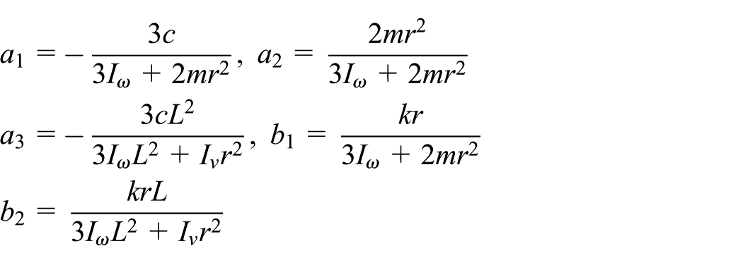
The dynamic property of the DC motor is described as shown in equation (3), where the moment of inertia of the wheel is defined as $I_{\omega }$ , the viscous friction factor is denoted by c, the gain factor of the driving torque is given as k, the control torques of the OMR are denoted by ${\tau }_i$ , and the input disturbance torques of the OMR are denoted by $d_i(i=1,2,3)$ . It should be noted that the viscous friction c is not easy to measure accurately, which is the key factor generating the uncertainty. In this article, all the driving wheels are assumed to have the same size and same characteristics

$$I_{\omega }{\stackrel{·}{\omega }}_i+c{\omega }_i=k({\tau }_i+d_i)-r{f}_i$$

(3)

The dynamics of the OMR can be derived with the similar process in Watanabe et al.’s ² work, and the force analysis of the OMR can be given as

$$\begin{array}{c}m({\stackrel{·}{v}}_x-v_y\stackrel{·}{\theta })=-\frac{1}{2}{f}_1-\frac{1}{2}{f}_2+f_3\hfill \\ m({\stackrel{·}{v}}_y+v_x\stackrel{·}{\theta })=\frac{\sqrt{3}}{2}{f}_1-\frac{\sqrt{3}}{2}{f}_2\hfill \\ I_v\stackrel{··}{\theta }=(f_1+f_2+f_3)L\hfill \end{array}$$

(4)

where m and $I_v$ denote the mass and moment of inertia of the OMR, respectively.

Then, the dynamic model can be written as

$$\begin{array}{c}\left(\begin{array}{c}{\stackrel{·}{v}}_x\hfill \\ \multicolumn{1}{c}{{\stackrel{·}{v}}_y}\\ \multicolumn{1}{c}{\stackrel{·}{\omega }}\end{array}\right)=\left(\begin{array}{c}{a}_1{v}_x\hfill \\ \multicolumn{1}{c}{a_1{v}_y}\\ \multicolumn{1}{c}{a_3\omega }\end{array}\right)+a_2\left(\begin{array}{c}\omega v_y\hfill \\ \multicolumn{1}{c}{-\omega v_x}\\ \multicolumn{1}{c}{0}\end{array}\right)\hfill \\ +\left(\begin{array}{ccc}-b_1\hfill & -b_1\hfill & 2b_2\hfill \\ \multicolumn{1}{c}{\sqrt{3}{b}_1}& -\sqrt{3}{b}_1\hfill & 0\hfill \\ \multicolumn{1}{c}{b_2}& b_2\hfill & b_2\hfill \end{array}\right)\left(\begin{array}{c}{\tau }_1+d_1\hfill \\ \multicolumn{1}{c}{{\tau }_2+d_2}\\ \multicolumn{1}{c}{{\tau }_3+d_3}\end{array}\right)\hfill \end{array}$$

(5)

where the parameters in the dynamic model are given as follows

$$\begin{array}{c}{a}_1=-\frac{3c}{3I_{\omega }+2m{r}^2},a_2=\frac{2m{r}^2}{3I_{\omega }+2m{r}^2}\hfill \\ a_3=-\frac{3c{L}^2}{3I_{\omega }{L}^2+I_v{r}^2},b_1=\frac{\mathrm{kr}}{3I_{\omega }+2m{r}^2}\hfill \\ b_2=\frac{\mathrm{krL}}{3I_{\omega }{L}^2+I_v{r}^2}\hfill \end{array}$$

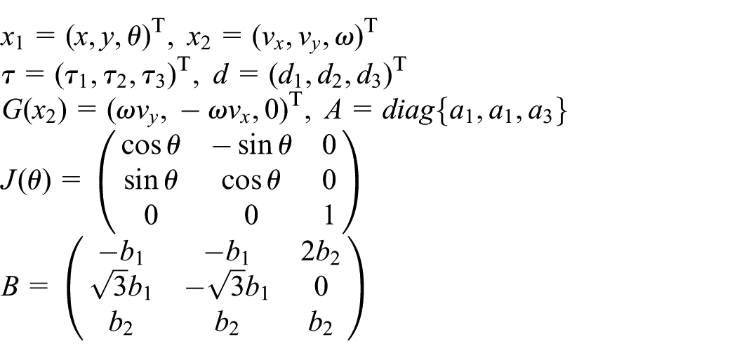
For the convenience of controller design, the kinematics and dynamics can be simplified as shown in equation (6)

$$\begin{array}{c}{\stackrel{·}{x}}_1=J(\theta )x_2\hfill \\ {\stackrel{·}{x}}_2=A{x}_2+a_{2}G(x_2)+B\tau +\mathrm{Bd}\hfill \end{array}$$

(6)

where

$$\begin{array}{c}{x}_1={(x,y,\theta )}^{\mathrm{T}},x_2={(v_x,v_y,\omega )}^{\mathrm{T}}\hfill \\ \multicolumn{1}{c}{\tau ={({\tau }_1,{\tau }_2,{\tau }_3)}^{\mathrm{T}},d={(d_1,d_2,d_3)}^{\mathrm{T}}}\\ \multicolumn{1}{c}{G(x_2)={(\omega v_y,-\omega v_x,0)}^{\mathrm{T}},A=\mathrm{diag}\{a_1,a_1,a_3\}}\\ \multicolumn{1}{c}{J(\theta )=\left(\begin{array}{ccc}\cos \theta \hfill & -\sin \theta \hfill & 0\hfill \\ \multicolumn{1}{c}{\sin \theta }& \cos \theta \hfill & 0\hfill \\ \multicolumn{1}{c}{0}& 0\hfill & 1\hfill \end{array}\right)}\\ \multicolumn{1}{c}{B=\left(\begin{array}{ccc}-b_1\hfill & -b_1\hfill & 2b_2\hfill \\ \multicolumn{1}{c}{\sqrt{3}{b}_1}& -\sqrt{3}{b}_1\hfill & 0\hfill \\ \multicolumn{1}{c}{b_2}& b_2\hfill & b_2\hfill \end{array}\right)}\end{array}$$

The control inputs cannot be infinite in the practical robot systems. Therefore, the input saturation can be expressed using the following constraints

$$\begin{array}{c}-{\tau }_{i_{\min }}⩽{\tau }_i⩽{\tau }_{i_{\max }},i=1,2,3\hfill \end{array}$$

(7)

where ${\tau }_{i_{\min }}$ and ${\tau }_{i_{\max }}$ are the known positive values. Thus, the control inputs can be defined as

$${\tau }_i=\mathrm{sat}({\tau }_{i_0})=\{\begin{array}{cc}{\tau }_{i_{\max }}\hfill & {\tau }_{i_0}>{\tau }_{i_{\max }}\hfill \\ \multicolumn{1}{c}{{\tau }_{i_0}}& {\tau }_{i_{\min }}⩽{\tau }_{i_0}⩽{\tau }_{i_{\max }}\hfill \\ \multicolumn{1}{c}{-{\tau }_{i_{\min }}}& {\tau }_{i_0}<-{\tau }_{i_{\min }}\hfill \end{array}$$

(8)

where ${\tau }_0=({\tau }_{1_0},{\tau }_{2_0},{\tau }_{3_0}{)}^{\mathrm{T}}$ is the unsaturated input torque to be designed. We define $\Delta \tau =\tau -{\tau }_0=(\Delta {\tau }_1,\Delta {\tau }_2,\Delta {\tau }_3{)}^{\mathrm{T}}$ .

The desired trajectory of the OMR is given as $x_{1d}=(x_d,y_d,{\theta }_d{)}^{\mathrm{T}}$ , and the desired speed of the robot is written as $x_{2d}=(v_{\mathrm{xd}},v_{\mathrm{yd}},{\omega }_d{)}^{\mathrm{T}}$ , which is related to the mathematical description of $x_{1d}$ and satisfies the kinematic equation (1). The objective of tracking control for the OMR is that the desired trajectory will be successfully tracked with all the state variables and control inputs meeting the constraints under the proposed control strategy.

In order to achieve the desired tracking performance of the robot, some lemmas and reasonable assumptions are introduced in this article.

Lemma 1

If a continuous and positive definite Lyapunov function $V(x)$ satisfies the condition ${\kappa }_1(\parallel x\parallel )⩽V(x)⩽{\kappa }_2(\parallel x\parallel )$ , such that $\stackrel{·}{V}(x)⩽-\mathrm{aV}(x)+b$ where a and b are positive constants and ${\kappa }_1,{\kappa }_2$ are K-class functions, the solution $x(t)$ will be uniformly bounded for any bounded initial state $x(t_0)$ . ¹⁹

Lemma 2

The following inequality will always hold for any $x\in R$ in the interval $|x|<|k|$ . ²¹

$$\log \frac{k^2}{k^2-x^2}⩽\frac{x^2}{k^2-x^2}$$

Lemma 3

For any positive constant $\varsigma >0$ and $x\in R$ , the inequality $|x|-x\tanh (\varsigma x)⩽\mu /\varsigma$ will always hold, where $\mu$ is a constant and satisfies $\mu =e^{-(\mu +1)}$ , that is, $\mu \approx 0.2785$ . ²⁵

Assumption 1

There exists an unknown constant $d^{*}$ such that $\parallel d\parallel ⩽d^{*}$ .

Assumption 2

The desired trajectories are given as $x_{1d}$ and $x_{2d}$ with the conditions $|x_{1\mathrm{di}}|<p_i$ and $|x_{2\mathrm{di}}|<q_i$ , where $p_i$ , $q_i(i=1,2,3)$ are the positive constants. All the elements in ${\stackrel{··}{x}}_{1d}=({\stackrel{··}{x}}_d,{\stackrel{··}{y}}_d,{\stackrel{··}{\theta }}_d{)}^{\mathrm{T}}$ are bounded. Moreover, the full-state constraints can be denoted by $|x_{1i}|<k_{c1i}$ , $|x_{2i}|<k_{c2i}$ , where $k_{c1i}$ , $k_{c2i}(i=1,2,3)$ are the positive constants satisfying $k_{c1i}>p_i,k_{c2i}>q_i$ .

Remark 1

In the practical system, Assumption 2 is reasonable and common, which implies that the state constraints of the trajectory and the robot always exist in the tracking process. The condition $k_{c1i}>p_i,k_{c2i}>q_i(i=1,2,3)$ means that the state boundary of the tracking OMR should be larger than the desired trajectory.

Controller design

In this part, an NN-based adaptive DSC method for the full-state constrained OMR system (5) subject to input saturation (equation (7)) will be established. The BLF is used to cope with the full-state constraints of the OMR, and the radial basis function (RBF) NN is employed to approximate system nonlinear dynamics. All signals in the OMR can be uniformly bounded.

• Step 1. Denote by $z_1=x_1-x_{1d}=(z_{11},z_{12},z_{13}{)}^{\mathrm{T}}$ the tracking error, where

$$\begin{array}{c}{z}_{11}=x-x_d\hfill \\ \multicolumn{1}{c}{z_{12}=y-y_d}\\ \multicolumn{1}{c}{z_{13}=\theta -{\theta }_d}\end{array}$$

(9)

Its derivative can be given by

$${\stackrel{·}{z}}_1=J(\theta )x_2-({\stackrel{·}{x}}_d,{\stackrel{·}{y}}_d,{\stackrel{·}{\theta }}_d{)}^{\mathrm{T}}$$

(10)

A virtual variable ${\alpha }_1=({\alpha }_{11},{\alpha }_{12},{\alpha }_{13}{)}^{\mathrm{T}}$ is proposed as

$${\alpha }_1=J(\theta {)}^{\mathrm{T}}[\left(\begin{array}{c}{\stackrel{·}{x}}_d\hfill \\ \multicolumn{1}{c}{{\stackrel{·}{y}}_d}\\ \multicolumn{1}{c}{{\stackrel{·}{\theta }}_d}\end{array}\right)-\left(\begin{array}{c}{k}_{a1}{z}_{11}\hfill \\ \multicolumn{1}{c}{k_{a2}{z}_{12}}\\ \multicolumn{1}{c}{k_{a3}{z}_{13}}\end{array}\right)]$$

(11)

where $k_{\mathrm{ai}}(i=1,2,3)$ is a positive constant.

A new variable $z_2=(z_{21},z_{22},z_{23}{)}^{\mathrm{T}}$ can be written as

$$z_2=x_2-{\alpha }_1$$

(12)

Substituting equation (12) into equation (10) will lead to

$${\stackrel{·}{z}}_1=J(\theta )z_2+J(\theta ){\alpha }_1-({\stackrel{·}{x}}_d,{\stackrel{·}{y}}_d,{\stackrel{·}{\theta }}_d{)}^{\mathrm{T}}$$

(13)

A BLF candidate is chosen as

$$V_1=\frac{1}{2}\sum _{i=1}^3\log \frac{k_{1i}^2}{k_{1i}^2-z_{1i}^2}$$

(14)

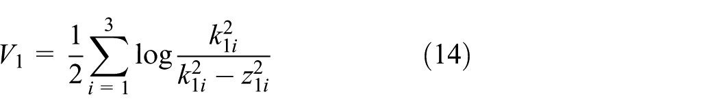
where $k_{1i}=k_{c1i}-p_i(i=1,2,3)$ is the positive constant. $V_1$ is continuous and positive definite. Combining with equations (11) and (13), we can get

$$\begin{array}{c}\multicolumn{1}{c}{\stackrel{·}{V}=\sum _{i=1}^3{\frac{z_{1i}{\stackrel{·}{z}}_{1i}}{k_{1i}^2-z_{1i}^2}}_1}\\ =-\sum _{i=1}^3\frac{k_{\mathrm{ai}}{z}_{1i}^2}{k_{1i}^2-z_{1i}^2}+\sum _{i=1}^3\frac{z_{1i}{J}_i(\theta )z_2}{k_{1i}^2-z_{1i}^2}\hfill \end{array}$$

(15)

• Step 2. Another BLF candidate can be chosen as

$$V_2=V_1+\frac{1}{2}\sum _{i=1}^3\log \frac{k_{2i}^2}{k_{2i}^2-z_{2i}^2}$$

(16)

where $k_2=(k_{21},k_{22},k_{23}{)}^{\mathrm{T}}$ is the positive constant vector and its value will be discussed later.

Differentiating $z_2$ , we can obtain

$${\stackrel{·}{z}}_2={\stackrel{·}{x}}_2-{\stackrel{·}{\alpha }}_{1d}=A{x}_2+a_{2}G(x_2)-{\stackrel{·}{\alpha }}_1+B\tau +\mathrm{Bd}$$

(17)

As a well-known fact, RBF NN can approximate an unknown continuous nonlinear dynamics with arbitrary precision and the mathematical description can be given as $\mathrm{\Gamma }(x_2)=W^{\mathrm{T}}S(x_2)+\delta$ , where W is the unknown optimal constant weight vector which will be adjusted by the adaptive law according to the analytical purpose, $S(x_2)$ is the vector consisting of RBF, and $\delta$ is the approximation error. The structure of the RBF NN is shown in Figure 2. For this matter, the RBF NN is employed to approximate $\mathrm{\Gamma }=A{x}_2+a_{2}G(x_2)$ as follows

$$\begin{array}{c}\mathrm{\Gamma }=\left(\begin{array}{c}{\mathrm{\Gamma }}_1\hfill \\ \multicolumn{1}{c}{{\mathrm{\Gamma }}_2}\\ \multicolumn{1}{c}{{\mathrm{\Gamma }}_3}\end{array}\right)=\left(\begin{array}{c}{W}_1^{\mathrm{T}}{S}_1+{\delta }_1\hfill \\ \multicolumn{1}{c}{W_2^{\mathrm{T}}{S}_2+{\delta }_2}\\ \multicolumn{1}{c}{W_3^{\mathrm{T}}{S}_3+{\delta }_3}\end{array}\right)\hfill \end{array}$$

(18)

Figure 2.

The schematic of the RBF NN structure.

The basis function can be chosen as

$$\begin{array}{c}{S}_{\mathrm{ij}}=\exp \left(\frac{-{(x_2-{\mu }_j)}^{\mathrm{T}}(x_2-{\mu }_j)}{{\sigma }_j^2}\right),\hfill \\ i=1,2,3;j=1,\dots ,N\hfill \end{array}$$

where $x_2=(x_{21},x_{22},x_{23}{)}^{\mathrm{T}}$ and the approximation errors satisfy the bounded conditions $\left|{\delta }_i\right|⩽{\delta }_i^{*}$ .

Denote by ${\hat{W}}_i$ the estimation of the ideal weight, and the error between the estimation and the optimal weight is expressed as ${\tilde{W}}_i=W_i-{\hat{W}}_i$ .

In equation (17), the differentiation of the virtual variable ${\alpha }_1$ will result in the complexity of the calculation, especially when the system order increases. Thus, the second-order sliding mode differentiator (equation (19)) is used as the dynamic surface to avoid the explosion of complexity and the derivative of ${\alpha }_1$ can be obtained in finite time

$$\begin{array}{c}{\stackrel{·}{\phi }}_1={\iota }_1\hfill \\ \multicolumn{1}{c}{{\iota }_1=-r_1|{\phi }_1-{\alpha }_1{|}^{\frac{1}{2}}\mathrm{sign}({\phi }_1-{\alpha }_1)+{\phi }_2}\\ \multicolumn{1}{c}{{\stackrel{·}{\phi }}_2=-r_2\mathrm{sign}({\phi }_1-{\alpha }_1)}\end{array}$$

(19)

where ${\phi }_1$ and ${\phi }_2$ are the state variables of the second-order finite time filter and $r_1$ and $r_2$ are the positive constants. From Levant’s ³⁶ previous work, ${\phi }_1$ and ${\iota }_1$ will converge to the virtual variable ${\alpha }_1$ and its derivative ${\stackrel{·}{\alpha }}_1$ in finite time, respectively, when there are no effects on the input signal ${\alpha }_1$ by noises. If the input signal including the external noise satisfies the condition $|{\alpha }_{1n}-{\alpha }_1|⩽\kappa$ , where $\kappa$ is the unknown constant and ${\alpha }_{1n}$ is the input signal with noise, we have $|{\iota }_1-{\stackrel{·}{\alpha }}_1|⩽\epsilon$ with $\epsilon$ being an unknown positive constant related to the values of $\kappa ,r_1,r_2$ .

Denote by $\hat{\epsilon }$ the estimation of the unknown constant $\epsilon$ and $\tilde{\epsilon }=\epsilon -\hat{\epsilon }$ .

Remark 2

If the initial states of the second-order differentiator satisfy $|{\phi }_1(0)-{\alpha }_1(0)|$ and $|{\phi }_2(0)-{\stackrel{·}{\alpha }}_1(0)|$ which are bounded, we can obtain ${\stackrel{·}{\alpha }}_1$ with arbitrary precision. It should be mentioned that we use the second-order finite time differentiator as the dynamic surface to overcome the explosion of complexity. In contrast to the conventional DSC where the first-order filter is adopted, poor precision can be avoided and finite time convergence can be achieved.

Differentiating $V_2$ , we obtain

$${\stackrel{·}{V}}_2={\stackrel{·}{V}}_1+\sum _{i=1}^3\frac{z_{2i}{\stackrel{·}{z}}_{2i}}{k_{2i}^2-z_{2i}^2}$$

(20)

In order to simplify the representation of the derivation procedure, we define

$$k{z}_{2i}=\frac{z_{2i}}{k_{2i}^2-z_{2i}^2}$$

Thus, we can obtain equation (21)

$${\stackrel{·}{V}}_2={\stackrel{·}{V}}_1+\sum _{i=1}^{3}k{z}_{2i}(W_i^{\mathrm{T}}{S}_i+{\delta }_i-{\stackrel{·}{\alpha }}_{1i}+B_i\tau +B_{i}d)$$

(21)

The following inequality can be deduced

$$k{z}_{2i}{\delta }_i⩽\frac{{\mathrm{kz}}_{2i}^2}{2k_{\delta }}+\frac{k_{\delta }{({\delta }_i)}^2}{2}$$

(22)

where $k_{\delta }$ is the positive constant.

To handle the input constraints, the auxiliary system is designed as

$${\stackrel{·}{\chi }}_i=(-k_{3i}+\frac{k_{4i}}{k_{2i}^2-z_{2i}^2}){\chi }_i+\Delta {\tau }_i,i=1,2,3$$

(23)

where $k_{3i}$ and $k_{4i}$ are the positive constants and $\Delta {\tau }_i={\tau }_i-{\tau }_{i_0}$ . Define the vector $\chi =({\chi }_1,{\chi }_2,{\chi }_3{)}^{\mathrm{T}}$ .

Then, we can get $k{z}_{2i}{B}_i\tau =k{z}_{2i}{B}_i{\tau }_0+k{z}_{2i}{B}_i\Delta \tau$ , and it is obvious to obtain the inequality as follows

$$k{z}_{2i}{B}_i\Delta \tau ⩽\frac{k{z_{2i}}^2}{2k_{\tau }}+\frac{k_{\tau }{\Vert B_i\Vert }^2{\Vert \Delta \tau \Vert }^2}{2}$$

(24)

where $k_{\tau }$ is a positive real constant and a small $k_{\tau }$ will be recommended.

Define $\mathrm{Bd}=\left(\begin{array}{c}{D}_1\hfill \\ \multicolumn{1}{c}{D_2}\\ \multicolumn{1}{c}{D_3}\end{array}\right)$ , and based on Assumption 2 we notice that there must exist unknown constants ${\tilde{d}}_i^{*}$ such that $|D_i|⩽{\tilde{d}}_i^{*}(i=1,2,3)$ . Then, we have

$$k{z}_{2i}{D}_i⩽\frac{{\mathrm{kz}}_{2i}^2}{2k_d}+\frac{k_d{({\tilde{d}}_i^{*})}^2}{2}$$

(25)

where $k_d$ is given as a positive constant and the smaller value of $k_d$ will decrease the influence of the disturbance.

Thus, the tracking controller can be given as

$$\begin{array}{c}\tau =\mathrm{sat}({\tau }_0)\hfill \\ {\tau }_0=-B^{-1}[K_b(z_2-\chi )+h-{\iota }_1+h_{\epsilon }\hfill \\ +(\frac{1}{2k_d}+\frac{1}{2k_{\tau }}+\frac{1}{2k_{\delta }}){(k{z}_{21},k{z}_{22},k{z}_{23})}^{\mathrm{T}}\hfill \\ +{({\hat{W}}_1^{\mathrm{T}}{S}_1,{\hat{W}}_2^{\mathrm{T}}{S}_2,{\hat{W}}_3^{\mathrm{T}}{S}_3)}^{\mathrm{T}}]\hfill \end{array}$$

(26)

where $K_b=\mathrm{diag}\{k_{b1},k_{b2},k_{b3}\}$ in which $k_{\mathrm{bi}}(i=1,2,3)$ are the positive constants, ${\iota }_1=({\iota }_{11},{\iota }_{12},{\iota }_{13}{)}^{\mathrm{T}}$ can be obtained from the second-order differentiator (equation (19)), $h_{\epsilon }=({\hat{\epsilon }}_1\tanh (\varsigma k{z}_{21}),{\hat{\epsilon }}_2\tanh (\varsigma k{z}_{22}),{\hat{\epsilon }}_3\tanh (\varsigma k{z}_{23}){)}^{\mathrm{T}}$ , and $h=(h_1,h_2,h_3{)}^{\mathrm{T}}$ is the vector described as

$$\begin{array}{c}{h}_1=(k_{21}^2-z_{21}^2)(\frac{z_{11}\cos \theta }{k_{11}^2-z_{11}^2}+\frac{z_{12}\sin \theta }{k_{12}^2-z_{12}^2})\hfill \\ h_2=(k_{22}^2-z_{22}^2)(-\frac{z_{11}\sin \theta }{k_{11}^2-z_{11}^2}+\frac{z_{12}\cos \theta }{k_{12}^2-z_{12}^2})\hfill \\ h_3=\frac{z_{13}(k_{23}^2-z_{23}^2)}{k_{13}^2-z_{13}^2}\hfill \end{array}$$

(27)

Differentiating $V_2$ will deduce equation (28) with the controller

$$\begin{array}{c}\multicolumn{1}{c}{{\stackrel{·}{V}}_2⩽-\sum _{i=1}^3\frac{k_{\mathrm{ai}}{z}_{1i}^2}{k_{1i}^2-z_{1i}^2}-\sum _{i=1}^3\frac{k_{\mathrm{bi}}{z}_{2i}^2}{k_{2i}^2-z_{2i}^2}+\sum _{i=1}^3\frac{k_{\mathrm{bi}}{z}_{2i}{\chi }_i}{k_{2i}^2-z_{2i}^2}}\\ +\sum _{i=1}^{3}k{z}_{2i}{{\tilde{W}}_i}^T{S}_i+\sum _{i=1}^{3}k{z}_{2i}({\iota }_{1i}-{\alpha }_{1i})\hfill \\ -\sum _{i=1}^{3}k{z}_{2i}{\hat{\epsilon }}_i\tanh (\varsigma k{z}_{2i})\hfill \\ +\sum _{i=1}^3\frac{k_{\tau }{\Vert B_i\Vert }^2{\Vert \Delta {\tau }_i\Vert }^2+k_{\delta }|{\delta }_i{|}^2+k_d{({\tilde{d}}_i^{*})}^2}{2}\hfill \end{array}$$

(28)

The adaptive laws for ${\hat{W}}_i$ and ${\hat{\epsilon }}_i$ are constructed by

$$\begin{array}{c}{\stackrel{·}{\hat{W}}}_i={\rho }_W(-{\lambda }_W{\hat{W}}_i+k{z}_{2i}{S}_i)\hfill \\ {\stackrel{·}{\hat{\epsilon }}}_i={\rho }_{\epsilon }[-{\lambda }_{\epsilon }{\hat{\epsilon }}_i+k{z}_{2i}\tanh (\varsigma k{z}_{2i})]\hfill \end{array}$$

(29)

where ${\rho }_W$ , ${\rho }_{\epsilon }$ , ${\lambda }_W$ , and ${\lambda }_{\epsilon }$ are the positive constants.

• Step 3. A new BLF candidate is given as

$$V=V_2+\frac{1}{2}{\chi }^{\mathrm{T}}\chi +\frac{1}{2{\rho }_W}\sum _{i=1}^3{\tilde{W}}_i^{\mathrm{T}}{\tilde{W}}_i+\frac{1}{2{\rho }_{\epsilon }}\sum _{i=1}^3{\tilde{\epsilon }}_i^2$$

(30)

Differentiating V, we have

$$\stackrel{·}{V}={\stackrel{·}{V}}_2+\sum _{i=1}^3{\chi }_i{\stackrel{·}{\chi }}_i-\frac{1}{{\rho }_W}\sum _{i=1}^3{\tilde{W}}_i^{\mathrm{T}}\stackrel{·}{\widehat{W_i}}-\frac{1}{{\rho }_{\epsilon }}\sum _{i=1}^3{\tilde{\epsilon }}_i\stackrel{·}{\widehat{{\epsilon }_i}}$$

(31)

Substituting equations (23), (28), and (29) into $\stackrel{·}{V}$ , we can obtain

$$\begin{array}{c}\stackrel{·}{V}⩽-\sum _{i=1}^3\frac{k_{\mathrm{ai}}{z}_{1i}^2}{k_{1i}^2-z_{1i}^2}-\sum _{i=1}^3\frac{k_{\mathrm{bi}}{z}_{2i}^2}{k_{2i}^2-z_{2i}^2}+\sum _{i=1}^3\frac{k_{\mathrm{bi}}{z}_{2i}{\chi }_i}{k_{2i}^2-z_{2i}^2}\hfill \\ \multicolumn{1}{c}{+\sum _{i=1}^3|k{z}_{2i}||{\iota }_{1i}-{\stackrel{·}{\alpha }}_{1i}|-\sum _{i=1}^{3}k{z}_{2i}{\epsilon }_i\tanh (\varsigma k{z}_{2i})}\\ \multicolumn{1}{c}{-\sum _{i=1}^3{k}_{3i}{\chi }_i^2-\sum _{i=1}^3\frac{k_{4i}}{k_{2i}^2-z_{2i}^2}{\chi }_i^2+\sum _{i=1}^3\Delta {\tau }_i{\chi }_i}\\ \multicolumn{1}{c}{+{\lambda }_W\sum _{i=1}^3{\tilde{W}}_i^{\mathrm{T}}{\hat{W}}_i+{\lambda }_{\epsilon }\sum _{i=1}^3{\tilde{\epsilon }}_i{\hat{\epsilon }}_i}\\ \multicolumn{1}{c}{+\sum _{i=1}^3\frac{k_{\tau }{\Vert B_i\Vert }^2{\Vert \Delta {\tau }_i\Vert }^2+k_{\delta }|{\delta }_i{|}^2+k_d{({\tilde{d}}_i^{*})}^2}{2}}\end{array}$$

(32)

The following inequalities will hold based on Young’s inequality

$$\frac{k_{\mathrm{bi}}{z}_{2i}{\chi }_i}{k_{2i}^2-z_{2i}^2}⩽\frac{k_{\mathrm{bi}}{z}_{2i}^2}{2(k_{2i}^2-z_{2i}^2)}+\frac{k_{\mathrm{bi}}{\chi }_i^2}{2(k_{2i}^2-z_{2i}^2)}$$

(33)

$$\Delta {\tau }_i{\chi }_i⩽\frac{\Delta {\tau }_i^2}{2}+\frac{{\chi }_i^2}{2}$$

(34)

$${{\tilde{W}}_i}^T{\hat{W}}_i⩽-\frac{{\Vert W_i\Vert }^2}{2}+\frac{{\Vert W_i\Vert }^2}{2}$$

(35)

$${\tilde{\epsilon }}_i{\hat{\epsilon }}_i⩽-\frac{{\tilde{\epsilon }}_i^2}{2}+\frac{{\epsilon }_i^2}{2}$$

(36)

Considering $|{\iota }_{1i}-{\stackrel{·}{\alpha }}_{1i}|⩽{\epsilon }_i$ and Lemma 3, we can deduce the following inequality

$$|k{z}_{2i}||{\iota }_{1i}-{\stackrel{·}{\alpha }}_{1i}|-k{z}_{2i}{\epsilon }_i\tanh (\varsigma k{z}_{2i})⩽\frac{\mu {\epsilon }_i}{\varsigma }$$

(37)

Substituting equations (33)–(37) into equation (32), then we have

$$\begin{array}{c}\stackrel{·}{V}⩽-\sum _{i=1}^3\frac{k_{\mathrm{ai}}{z}_{1i}^2}{k_{1i}^2-z_{1i}^2}-\sum _{i=1}^3\frac{k_{\mathrm{bi}}{z}_{2i}^2}{2(k_{2i}^2-z_{2i}^2)}\hfill \\ \multicolumn{1}{c}{-\sum _{i=1}^3(k_{3i}-\frac{1}{2}){\chi }_i^2-\frac{{\lambda }_W}{2}\sum _{i=1}^3{\Vert W_i\Vert }^2}\\ \multicolumn{1}{c}{-\frac{{\lambda }_{{\epsilon }_i}}{2}\sum _{i=1}^3{\tilde{\epsilon }}_i^2+\sum _{i=1}^3(\frac{k_{\mathrm{bi}}}{2}-k_{4i})\frac{{\chi }_i^2}{k_{2i}^2-z_{2i}^2}}\\ \multicolumn{1}{c}{+\frac{1}{2}\sum _{i=1}^3[\Delta {\tau }_i^2+\frac{2\mu {\epsilon }_i}{\varsigma }+{\lambda }_W{\Vert W_i\Vert }^2+{\lambda }_{\epsilon }{{\epsilon }_i}^2}\\ \multicolumn{1}{c}{+k_{\tau }{\Vert B_i\Vert }^2{\Vert \Delta {\tau }_i\Vert }^2+k_{\delta }|{\delta }_i{|}^2+k_d{({\tilde{d}}_i^{*})}^2]}\end{array}$$

(38)

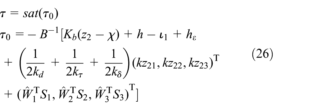
It is worth mentioning that the magnitude of $\Delta {\tau }_i$ should be bounded by an unknown positive constant in the practical system. If $\Delta {\tau }_i$ becomes infinite, it means that the desired trajectory cannot be tracked by the OMR which is far beyond the capabilities of the robot. Thus, it is reasonable to assume that $\Delta {\tau }_i$ is bounded for the stability of the closed-loop system. As a matter of fact, the effects caused by input saturation can be compensated with the auxiliary system (equation (23)). When the input difference $\Delta {\tau }_i$ between the actual actuator output and unsaturated output is not equal to zero, ${\chi }_i$ will be used in the controller (equation (26)) to reduce the adverse effects of the input constraints until $\Delta {\tau }_i=0$ .

Theorem 1

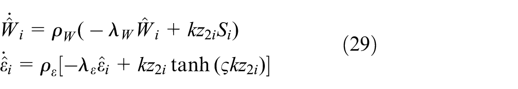
Consider the OMR system (equation (5)) with full-state constraints under Assumptions 1 and 2. If the initial states of $z_{1i}(0)$ and $z_{2i}(0)$ stay in the bounded area as ${\Delta }_1\stackrel{\Delta }{=}\{|z_{1i}|<k_{1i},i=1,2,3\}$ and ${\Delta }_2\stackrel{\Delta }{=}\{|z_{2i}|<k_{2i},i=1,2,3\}$ , respectively, then an NN-based adaptive dynamic surface controller (equation (26)) and the adaptive law (equation (29)) are given, which can guarantee that all signals $\{z_{1i},z_{2i},x_1,x_2,{\hat{W}}_i,\hat{\epsilon },{\chi }_i,{\alpha }_i,{\iota }_{1i}\}$ in the closed-loop system are uniformly bounded, if the condition in equation (39) holds. The state variables $x_{1i}$ and $x_{2i}$ in system (5) will always remain in the sets ${\Omega }_1\stackrel{\Delta }{=}\{|x_{1i}|<k_{c1i},i=1,2,3\}$ and ${\Omega }_2\stackrel{\Delta }{=}\{|x_{2i}|<k_{c2i},i=1,2,3\}$ with suitable parameters. $z_{1i}$ and $z_{2i}$ will converge to sufficiently small compacts of zero with suitable parameters

$$\begin{array}{c}{k}_{\mathrm{ai}}>0,k_{\mathrm{bi}}>0,k_{3i}>\frac{1}{2}\hfill \\ 0<k_{4i}⩽\frac{k_{\mathrm{bi}}}{2},i=1,2,3\hfill \\ {\lambda }_W>0,{\lambda }_{\epsilon }>0\hfill \end{array}$$

(39)

Proof

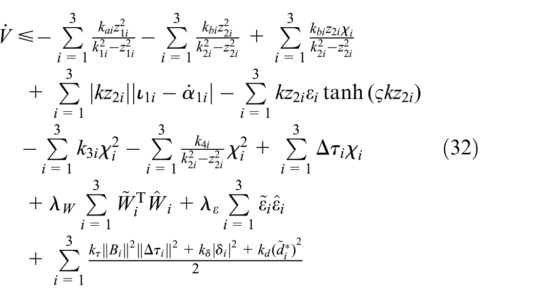
If the condition in equation (39) holds, then the inequality in equation (38) can be described based on Lemma 1 as follows

$$\stackrel{·}{V}⩽-\mathrm{aV}+b$$

(40)

where a is the positive constant which can be written as

$$\begin{array}{l}a=\underset{i=1,2,3}{{\displaystyle \min }}\{2k_{ai},k_{bi},2k_{3i}-1,{\rho }_W{\lambda }_W,{\rho }_{\epsilon }{\lambda }_{\epsilon }\}\hfill \end{array}$$

(41)

and b is given as

$$\begin{array}{c}\multicolumn{1}{c}{b=\frac{1}{2}\sum _{i=1}^3[\Delta {\tau }_i^2+\frac{2\mu {\epsilon }_i}{\varsigma }+{\lambda }_W{\Vert W_i\Vert }^2+{\lambda }_{\epsilon }{\epsilon }_i^2}\\ \multicolumn{1}{c}{+k_{\tau }{\Vert B_i\Vert }^2{\Vert \Delta {\tau }_i\Vert }^2+k_{\delta }|{\delta }_i{|}^2+k_d{({\tilde{d}}_i^{*})}^2]}\end{array}$$

(42)

Thus, solving the differential inequality in equation (40), we can deduce the inequality as follows

$$V(t)⩽[V(0)-\frac{b}{a}]e^{-\mathrm{at}}+\frac{b}{a}$$

(43)

where $V(0)$ is the initial state which is related with $z_1(0)$ and $z_2(0)$ .

Moreover, it is easy to obtain

$$\underset{t\to \infty }{lim}V(t)⩽\frac{b}{a}$$

which means that the convergence domain will be sufficiently small with large a and small b. To be specific, a will be large when $k_{\mathrm{ai}}$ , $k_{\mathrm{bi}}$ , $k_{3i}$ , $k_{\mathrm{ai}}$ , ${\rho }_W$ , and ${\rho }_{\epsilon }$ are large, and b will be small as long as $k_{\tau }$ , $k_d$ , $k_{\sigma }$ , ${\lambda }_W$ , ${\lambda }_{\epsilon }$ , and ${\delta }^{*}$ are small.

We can obtain equation (44) from equation (43)

$$\begin{array}{c}\frac{1}{2}\sum _{i=1}^3\log \frac{k_{1i}^2}{k_{1i}^2-z_{1i}^2}+\frac{1}{2}\sum _{i=1}^3\log \frac{k_{2i}^2}{k_{2i}^2-z_{2i}^2}\hfill \\ ⩽[V(0)-\frac{b}{a}]e^{-\mathrm{at}}+\frac{b}{a}\hfill \end{array}$$

(44)

It is obvious to get

$$\begin{array}{c}\multicolumn{1}{c}{\frac{1}{2}\log \frac{k_{1i}^2}{k_{1i}^2-z_{1i}^2}⩽[V(0)-\frac{b}{a}]e^{-\mathrm{at}}+\frac{b}{a}}\\ \multicolumn{1}{c}{\frac{1}{2}\log \frac{k_{2i}^2}{k_{2i}^2-z_{2i}^2}⩽[V(0)-\frac{b}{a}]e^{-\mathrm{at}}+\frac{b}{a}}\end{array}$$

(45)

Accordingly, solving the inequality, the compacts of $z_{1i}$ and $z_{2i}$ can be written as

$$\begin{array}{c}\multicolumn{1}{c}{|z_{1i}|⩽k_{1i}\sqrt{1-e^{-2[(V(0)-\frac{b}{a})e^{-\mathrm{at}}+\frac{b}{a}]}}<k_{1i}}\\ \multicolumn{1}{c}{|z_{2i}|⩽k_{2i}\sqrt{1-e^{-2[(V(0)-\frac{b}{a})e^{-\mathrm{at}}+\frac{b}{a}]}}<k_{2i}}\end{array}$$

(46)

Now, we discuss the boundedness of $x_1$ and $x_2$ . As we mentioned above, $k_{1i}$ is defined as $k_{1i}=k_{c1i}-p_i$ . From $z_{1i}=x_{1i}-x_{1\mathrm{di}}$ , $|x_{1i}|<|z_{1i}|+|x_{1\mathrm{di}}|<k_{c1i}$ will hold, which satisfies the constraint of $x_{1i}(i=1,2,3)$ . According to equation (11), we can deduce the equation as ${\alpha }_1=x_{2d}-J(\theta {)}^{\mathrm{T}}{K}_a{z}_1$ , where $K_a=\mathrm{diag}\{k_{a1},k_{a2},k_{a3}\}$ . Based on $\parallel J(\theta {)}^{\mathrm{T}}\parallel ⩽3$ , we have $|{\alpha }_{1i}{|}_{\max }<q_i+3k_{\mathrm{ai}}{k}_{1i}$ . Therefore, if $k_{2i}$ satisfies the condition $k_{2i}=k_{c2i}-q_i-3k_{\mathrm{ai}}{k}_{1i}$ , the constraint $|x_{2i}|<k_{c2i}$ will hold. The boundedness of other signals such as ${\hat{W}}_i$ , $\hat{\epsilon }$ , ${\chi }_i$ , and ${\iota }_{1i}$ in the closed-loop system can be proved to be uniformly bounded with the similar process. The proof is complete.

Remark 3

It should be mentioned that the convergence compact of $V(t)$ is bounded up with $b/a$ , and the value of $k_{2i}$ is given by magnification and shrinking of inequality with conservative property. On the one hand, larger a and smaller b are desired to make the domain of convergence sufficiently small, which could lead to larger $k_{\mathrm{ai}}$ . On the other hand, the value of $k_{2i}$ requires smaller $k_{\mathrm{ai}}$ . Thus, the value of $k_{\mathrm{ai}}$ should be chosen carefully. Actually, the value of $k_{2i}$ can be chosen bigger than the value calculated by $k_{2i}=k_{c2i}-q_i-3k_{\mathrm{ai}}{k}_{1i}$ because of the conservative property.

Remark 4

It is worth mentioning that the proposed adaptive DSC method based on NN is partly motivated by the previous work.^22,23 It should be pointed out that the proposed adaptive NN controllers^22,23 need the information of ${\stackrel{·}{\alpha }}_1$ , which may bring out the singularity or computational complexity. The dynamic surface adopted in this article has the advantage of avoiding the derivative of ${\alpha }_1$ , which simplifies the structure of the controller and reduces the calculated amount.

Remark 5

Note that the adaptive law of RBF NN uses the tracking errors to update the weights, which may cause poor transient performance. In this article, the BLF method is adopted to avoid the violation of state constraints, which can also ensure the transient performance as shown in equation (46). It should be pointed out that a novel predictor-based neural DSC scheme has been proposed, ²⁹ and better transient performance can be obtained by integrating a state predictor into the neural DSC method. For the OMR tracking problem, the predictor can be written as $\stackrel{·}{\widehat{x_1}}=x_2-(k_{p1}-{\kappa }_{p1}){\tilde{x}}_1$ and $\stackrel{·}{\widehat{x_2}}={\hat{W}}^{\mathrm{T}}S+B\tau -(k_{p2}-{\kappa }_{p2}){\tilde{x}}_2$ , and a similar process can be followed with the previous work.

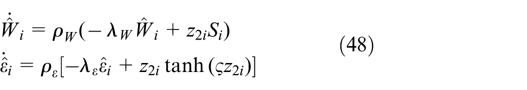
In order to verify the advantages of the BLF method and the anti-windup compensator, the traditional Lyapunov function $V_2=(z_1^2/2)+(z_2^2/2)$ is chosen to replace the BLF terms, then the unsaturated adaptive neural DSC scheme for trajectory tracking of the OMR is proposed as follows

$$\begin{array}{c}\multicolumn{1}{c}{\tau =-B^{-1}[K_b{z}_2+h_N-{\iota }_1+h_{\epsilon 2}}\\ +(\frac{1}{2k_d}+\frac{1}{2k_{\tau }}+\frac{1}{2k_{\delta }}){(z_{21},z_{22},z_{23})}^{\mathrm{T}}\hfill \\ +({\hat{W}}_1^{\mathrm{T}}{S}_1,{\hat{W}}_2^{\mathrm{T}}{S}_2,{\hat{W}}_3^{\mathrm{T}}{S}_3{)}^{\mathrm{T}}]\hfill \end{array}$$

(47)

where $h_{\epsilon 2}=({\hat{\epsilon }}_1\tanh (\varsigma z_{21}),{\hat{\epsilon }}_2\tanh (\varsigma z_{22}),{\hat{\epsilon }}_3\tanh (\varsigma z_{23}){)}^{\mathrm{T}}$ , and $h_N=(h_{N1},h_{N2},h_{N3}{)}^{\mathrm{T}}$ is the vector defined as $h_{N1}=z_{11}\cos \theta +z_{12}\sin \theta$ , $h_{N2}=-z_{11}\sin \theta +z_{12}\cos \theta$ , and $h_{N3}=z_{13}$ .

The adaptive laws for equation (47) are given as

$$\begin{array}{c}{\stackrel{·}{\hat{W}}}_i={\rho }_W(-{\lambda }_W{\hat{W}}_i+z_{2i}{S}_i)\hfill \\ {\stackrel{·}{\hat{\epsilon }}}_i={\rho }_{\epsilon }[-{\lambda }_{\epsilon }{\hat{\epsilon }}_i+z_{2i}\tanh (\varsigma z_{2i})]\hfill \end{array}$$

(48)

The comparison between controller equations (26) and (47) will be illustrated in the next part.

Numerical results

In this section, simulation experiments are proposed to illustrate the effectiveness and tracking performance of the NN-based adaptive DSC controller (equation (26)), and characteristic parameters of the OMR are given as $m=9.4\mathrm{kg}$ , $L=0.4\mathrm{m}$ , $k=1.0$ , $R=0.05\mathrm{m}$ , $I_v=11.25\mathrm{kg}{\mathrm{m}}^2$ , $I_w=0.04108\mathrm{kg}{\mathrm{m}}^2$ , and $c=0.02\mathrm{kg}{\mathrm{m}}^2/\mathrm{s}$ . The desired trajectories are defined as $x_{11d}=1.5\sin (0.1t)\mathrm{m}/\mathrm{s}$ , $x_{12d}=\sin (0.2t)\mathrm{m}/\mathrm{s}$ , and $x_{13d}=\sin (0.1t)\mathrm{rad}/\mathrm{s}$ . The constraints of $x_1$ and $x_2$ in the tracking process are defined as $k_{c1}=(2,1.5,1.5{)}^{\mathrm{T}}$ and $k_{c2}=(0.25,0.32,0.22{)}^{\mathrm{T}}$ , respectively. The initial states of the OMR are chosen by $x_1(0)=(0.4,-0.4,0.3{)}^{\mathrm{T}}$ and $x_2(0)=(0.1,0.1,0.1{)}^{\mathrm{T}}$ . Then, the parameters in controller (equation (26)) are chosen as follows: $k_{\mathrm{ai}}=0.1$ , $k_{\mathrm{bi}}=0.2$ , $k_{1i}=0.5$ , $k_{2i}=0.1$ , $k_{3i}=0.6$ , $k_{4i}=0.1$ , $k_d=k_{\tau }=k_{\delta }=0.5$ , and $\varsigma =5$ . The parameters of the second-order differentiator are set as $r_1=1.5$ and $r_2=1.1$ . The RBF NN $W_i^{\mathrm{T}}{S}_i(i=1,2,3)$ contain 10 nodes and the centers are uniformly distributed in the interval $[-2,2]$ with widths being equal to 4. The parameters of the adaptive law are defined as ${\rho }_{\epsilon }={\rho }_W=2$ and ${\lambda }_{\epsilon }={\lambda }_W=0.01$ . The initial states of adaptive parameters, the auxiliary system, and the differentiator are chosen as ${\hat{W}}_i(0)=\mathrm{zeros}(10,1)$ and ${\epsilon }_i(0)={\chi }_i(0)={\phi }_1(0)={\phi }_2(0)=0$ . The input disturbances are defined as $d_1=0.06-0.04\sin (t)+0.05\cos (t)$ , $d_2=0.03-0.02\sin (t)+0.01\cos (t)$ , and $d_3=0.05+0.05\sin (t)-0.02\cos (t)$ . The input constraints are defined by $-0.5\mathrm{N}\mathrm{m}=-{\tau }_{i_{\min }}⩽{\tau }_i⩽{\tau }_{i_{\max }}=0.5\mathrm{N}\mathrm{m}$ .

Figure 3 shows the tracking performance of the OMR with the controller (equation (26)), and Figure 4 shows the response trajectory of $x_2$ of the OMR with the proposed controller (equation (26)). It is obvious to observe that the OMR will track the desired trajectory satisfying the full-state constraints. Tracking errors of $z_1$ and $z_2$ are shown in Figure 5, which means that the signals of $z_1$ and $z_2$ will be uniformly bounded if the initial states stay in the compact. The RBF NN is used to estimate the unknown function $\mathrm{\Gamma }=A{x}_2+a_{2}G(x_2)$ , and the NN estimation of $\mathrm{\Gamma }$ is displayed in Figure 6. In addition, we demonstrate the adaptive law $\hat{\epsilon }$ , the output ${\iota }_1$ of the differentiator, the auxiliary system, and the control torques as shown in Figures 7 and 8, respectively. When the input difference $\Delta {\tau }_i\ne 0$ , the auxiliary system will work to compensate for the adverse effects because of input limits, until that the torques will never violate the boundary of input constraints. According to the above figures, we can conclude that both state constraints and input saturation will be followed under the controller (equation (26)). Finally, the actual trajectory in the tracking process and the desired trajectory of the OMR are also presented in Figure 9.

Figure 3.

Comparison between $x_1$ and $x_{1d}$ under the controller (equation (26)).

Figure 4.

Response trajectory of $x_2$ under the controller (equation (26)).

Figure 5.

Tracking errors of $z_1$ and $z_2$ under the controller (equation (26)).

Figure 6.

NN estimations of $\mathrm{\Gamma }$ under the controller (equation (26)).

Figure 7.

The adaptive law $\hat{\epsilon }$ and the output ${\iota }_1$ of the second-order differentiator.

Figure 8.

The state variable $\chi$ of the compensator (equation (23)) and the input torque $\tau$ under the controller (equation (26)).

Figure 9.

The comparison of the actual trajectory and the desired trajectory under the controller (equation (26)).

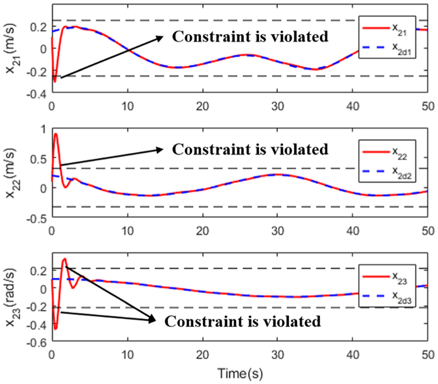
To further demonstrate the advantages of the proposed controller (equation (26)), the unsaturated adaptive controller (equation (47)), where the BLF term is replaced by the traditional Lyapunov function, is presented to contrast with equation (26). And all parameters are the same as in equation (26). The response trajectories of $x_1$ and $x_2$ , tracking errors of $z_1$ and $z_2$ , NN estimation of $\mathrm{\Gamma }$ , adaptive law of $\hat{\epsilon }$ , output ${\iota }_1$ of the second-order differentiator, and input torques ${\tau }_i$ are presented in Figures 10–14, respectively. As shown in Figure 11, the constraint of $x_{22}$ is clearly violated with the controller (equation (47)), which means that the full-state constraints cannot be achieved. It is easy to find that the transient performance of $z_1$ and $z_2$ in Figure 12 is worse than that under the controller (equation (26)). According to Figure 14, the control inputs under equation (47) are larger than those of equation (26), and its performance will degrade when actuators are subject to the input saturations.

Figure 10.

Comparison between $x_1$ and $x_{1d}$ under the controller (equation (47)).

Figure 11.

Response trajectory of $x_2$ under the controller (equation (47)).

Figure 12.

Tracking errors of $z_1$ and $z_2$ under the controller (equation (47)).

Figure 13.

NN estimations of $\mathrm{\Gamma }$ under the controller (equation (47)).

Figure 14.

The adaptive law $\hat{\epsilon }$ , the output ${\iota }_1$ of the second-order differentiator, and the input torques ${\tau }_i$ under the controller (equation (47)).

Moreover, a proportional–derivative (PD) controller ² $\tau =-B^{-1}(\mathrm{Kp}{z}_1+\mathrm{Kd}{\stackrel{·}{z}}_1)$ will also be used for comparison, where the control gains are given as $\mathrm{Kp}=\mathrm{diag}\{8,8,8\}$ and $\mathrm{Kd}=\mathrm{diag}\{3,2,1\}$ . The initial states and constraints of the state variables are the same as those in the above scenario. The simulation results with the PD controller are shown in Figures 15–18. We can see that, although the PD controller can guarantee that the tracking error $z_1$ converges to a sufficiently small value, the tracking performance of OMR is not as good as the proposed controller (equation (26)). It should be noticed that the state constraints of $x_{21}$ , $x_{22}$ , and $x_{23}$ will be violated during the tracking process. Meanwhile, the control inputs far exceed the input torque with the controller (equation (26)).

Figure 15.

Comparison between $x_1$ and $x_{1d}$ under the PD controller.

Figure 16.

Response trajectory of $x_2$ under the PD controller.

Figure 17.

Tracking error of $z_1$ under the PD controller.

Figure 18.

The control inputs ${\tau }_i$ under the PD controller.

Conclusion

In this article, the kinematics and dynamics of a three-wheeled OMR with uncertainty and input disturbance are discussed. The adaptive NN approximation technique is applied to estimate the unknown nonlinear dynamics and the BLF with error variables is employed to guarantee the constraints which are not violated. Moreover, the proposed DSC method can avoid the explosion of complexity problem for conventional backstepping. The auxiliary system is adopted to ensure that the input torque of the robot will satisfy the input saturation. Finally, the numerical simulation results verify that the OMR will track the desired trajectory with great performance by employing the NN-based adaptive dynamic surface controller we proposed. In the future work, time-varying state constraints, which are common in practical systems, should be taken into account, and the proposed algorithm will be developed with new techniques.