Sage Journals: Discover world-class research

Abstract

Reliability of steam generator is a serious concern in the operation of nuclear power plants, especially for steam generator tubes that experience a variety of degradation mechanisms including wear damage. It is necessary to develop a model to accurately predict wear depth of tubes for the assessment and management of steam generator aging. In this article, a non-homogeneous Markov process model of wear is proposed to assess the evaluation of wear depth in steam generator tubes. Based on the analytical solutions of the system of Kolmogorov’s forward equations, the transition probability functions are computed to estimate the future wear depth distribution. The parameters are estimated under the assumption that the mean wear depths in the proposed Markov stochastic model are equal to the average of measured depths. The time evolution of wear depth distribution can be predicted. The proposed Markov stochastic model was tested with the in-service inspection records from steam generator tube inspection report, and the results showed a good agreement with future wear depth distribution.

Keywords

Non-homogeneous Markov process time evolution wear depth steam generator tubes

Introduction

Steam generator (SG) tubes in nuclear power plants play an important safety role in transferring heat and isolating the radioactive products in the primary coolant from the secondary system. Ten-thousand U-shaped tubes are installed in a typical SG of pressurized water reactors, which are supported at intermediate points by tube support plates (TSPs) in the straight-leg region and by anti-vibration bars (AVBs) in the U-bend region.¹ Clearances between the tubes and TSPs or AVBs are designed for thermal expansion and manufacturing considerations. The presence of clearances permits the tubes to impact and slide when excited sufficiently by the flow, which can result in tube wear damage.^2,3 When the wear depth makes the remaining thickness of a tube lower than the minimum wall thickness criterion, the tube is required to be plugged. Therefore, it is important to evaluate the wear state of tubes during the long-term operation of SG.

The most used wear model for estimating the material losses due to wear is based on the relationship derived by Archard equation.⁴ In the model, the wear volume is considered as a linear function of local loads and sliding distances. The linear coefficient is called wear coefficient, which relies on not only the materials of tube and support but also the environmental conditions including coolant composition, temperature, and so on. Later, a parameter named as work rate is defined, which relates to local loads and sliding distances based on the energy dissipation.⁵ To predict the time history of the maximum wear depth of the tube, the wear coefficient and work rate should be obtained. Large number of research works can be found on the wear coefficient from the view point of material properties.^6,7 Not surprisingly, most results indicate that wear coefficient presents to be disperse, which not only affected by the material itself but also the service conditions.^8–10 Another challenge with wear depth evaluation is that it is hard to compute the work rate that depends on dynamic characteristics of SG tubes under multiphase fluid.¹¹ Therefore, it is difficult to evaluate the accurate wear depth on wear mechanism during the operation of nuclear power plants.

Recognizing these situations, a strategy for the assessment of SG tube integrity based on the theory of probability and statistics is studied and adopted in engineering practice.¹² The approach utilizes the data of in-service inspection (ISI) by non-destructive examination (NDE) to determine degradation growth rate, which is regarded as a random variable. An estimate of the 95th percentile growth rate using the empirical distribution is considered to be conservative in assessing SG tube integrity. Therefore, it is neither necessary to calculate the work rates of wear nor to obtain wear coefficients. In addition, statistical methodology has been used to predict the accumulated number of SG plugged tubes and the growth rate of wall thinning for the degraded SG tubes.^13,14 These statistical models consider relevant parameters as random variables, such as degradation growth rate and NDE sizing error. Then, the remaining wall thickness over time can be estimated on the degradation growth rate by Monte Carlo simulation. Although these statistical variable models can reflect the uncertainty of wear growth rate from the ISI data, it is difficult to give a systematic evolution of wear growth rate with the operation of nuclear power plant.

Statistical variable models are associated with or indexed by a set of numbers, usually viewed as points in time, while a stochastic process represents numerical values of some system randomly changing over time. Stochastic processes are widely used as mathematical models for modeling the degradation over time,¹⁵ for example, Wiener process,¹⁶ Gamma process,¹⁷ and inverse Gaussian process.¹⁸ For wear degradation, the remaining wall thickness over time can be regarded as a stochastic process. Wang et al.¹⁹ used a Wiener process model to fit the head wear data of hard disk drives. In particular, Markov chain–based models were widely utilized for degradation processes of systems with discrete states. Kharoufeh²⁰ characterized the cumulative wear by a non-decreasing stochastic process and modeled the environment process as a finite-state Markov process. Markov chain–based approaches^21–23 have been proposed for tool wear monitoring and tool life prediction.

For other degradation mechanism, the continuous-time Markov chain model has been widely used to predict pitting corrosion damage^24–26 and fatigue damage,^27,28 and it has shown to agree well with experimental results. In general, the pit growth process is treated as a non-homogeneous Markov process, in consideration of the time dependence of material’s corrosion rate. Recently, Xie et al.²⁹ developed a physics-based multi-state Markov model to describe pitting corrosion states including the initial state, growth state, declining state, repassivation state, and critical state.

In this article, Markov process is proposed to describe SG tube wear depth with time and assess the wear depth growth rate. A non-homogeneous Markov process model of wear is introduced. Some measured data sets are analyzed using the model. The stochastic model is able to predict the time evolution of the probability distribution of wear depths.

Markov stochastic process model of wear

Continuous-time Markov chain model

A continuous-time Markov chain model is considered to describe SG tube wear. As known that the future state of the Markov process depends on the current state, it is conditionally independent of the past states of the stochastic process. In other words, it is assumed that the increase in the wear depth at the end of a time interval (s, t) depends in a probabilistic manner only on the amount of wear depth present at the start of the interval s and on the interval itself (t–s).

Let ${D (t)}$ be a continuous-time Markov chain, the transition probability function $p_{i, j} (s, t)$ from state i to state j in the time interval (s, t) can be defined as

\begin{matrix} p_{i, j} (s, t) = \Pr {D (t) = j | D (s) = i}, & 0 \leq s < t \end{matrix}

(1)

assumed to be continuous at $t - s = 0$

lim_{t - s \to 0} p_{i, j} (s, t) = δ_{i, j} = {\begin{matrix} 1 & i = j \\ 0 & i \neq j \end{matrix}

(2)

For the tube wear process, the possible wear depths, as shown in Figure 1, constitute the Markov state space. The wall thickness is divided into N discrete Markov states. The wear depth at time t is represented by a discrete random variable D(t), considering the probability $p_{j} (t)$ that D(t) assumed state j, $\Pr {D (t) = j} = p_{j} (t)$ , with j = 1, 2,…, N. The wear depth distribution at any future moment t can be estimated using

p_{j} (t) = \sum_{i = 1}^{j} p_{i} (t_{0}) p_{i, j} (t_{0}, t)

(3)

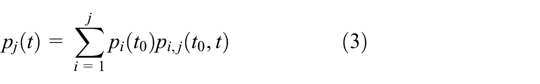
if the probability distribution of the wear depth at t₀ is known, that is, $\Pr {D (t_{0}) = i} = p_{i} (t_{0})$ .

Figure 1.

A sample path of a Markov process.

For the case of SG tube, the initial probability distribution of wear depths can be evaluated on the ISI data collected from regular inspection by non-destructive methods such as eddy current and ultrasonic. The ISI data can give information about location, volume, depth, length, and width of the wear. It is convenient to estimate the probability distribution from the ISI data with several wear depths D(t₀) at the inspection time t₀ on probability and statistical theory. Therefore, the key to determine the wear depth distribution at any future moment $p_{j} (t)$ is the transition probability $p_{i, j} (t_{0}, t)$ .

Transition probability

To obtain the transition probability functions of a continuous-time Markov chain, one usually solved a system of differential equations for the transition probability functions. A fundamental relation satisfied by the transition probability function of a Markov chain is the so-called Chapman–Kolmogorov equation: for any time $0 \leq s < u < t$ and states i and j

p_{i, j} (s, t) = \sum_{states k} p_{i, k} (s, u) p_{k, j} (u, t)

(4)

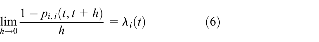
From the Chapman–Kolmogorov equation, one may derive various differential relations for the transition probability functions. Among these equations, Kolmogorov’s forward equation can describe as

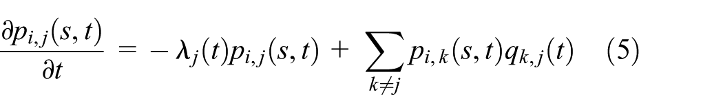
\frac{\partial p_{i, j} (s, t)}{\partial t} = - λ_{j} (t) p_{i, j} (s, t) + \sum_{k \neq j} p_{i, k} (s, t) q_{k, j} (t)

(5)

Given that the Markov chain is in state i at time t, $λ_{i} (t)$ is the intensity at which the process leaves the state, and $q_{i, j} (t)$ is called the transition intensity from state i to j. It is assumed that for each state i, there is a non-negative continuous function $λ_{i} (t)$ defined by the limit

lim_{h \to 0} \frac{1 - p_{i, i} (t, t + h)}{h} = λ_{i} (t)

(6)

and for each pair of states i and j (with $i \neq j$ ), there is a non-negative continuous function defined by the limit

lim_{h \to 0} \frac{p_{i, j} (t, t + h)}{h} = q_{i, j} (t)

(7)

One can obtain the transition probability functions from solving Kolmogorov’s forward equation. Parzen³⁰ solved the differential equation using the transition probability generating function

ψ_{i, s} (z, t) = \sum_{k = 0}^{N} z^{k} p_{i, k} (s, t)

(8)

defined for any state j, times s < t, and $| z | \leq 1$ .

Noting the physical process of wear, the wear state j transferring to a state i < j is impossible. The conditional probability of transition may depend on both the time of observing the process t and the current wear state i. Then, a non-homogeneous pure birth Markov process is considered to model the wear of SG tube with

\begin{matrix} q_{i, j} (t) = 0 & j \neq i or i + 1 \end{matrix}

(9)

For a pure birth process, Kolmogorov’s forward equation becomes

\frac{\partial p_{i, j} (s, t)}{\partial t} = - λ_{j} (t) p_{i, j} (s, t) + λ_{j - 1} (t) p_{i, j - 1} (s, t) j \geq i + 1

(10)

and

\frac{\partial p_{i, i} (s, t)}{\partial t} = - λ_{i} (t) p_{i, i} (s, t)

(11)

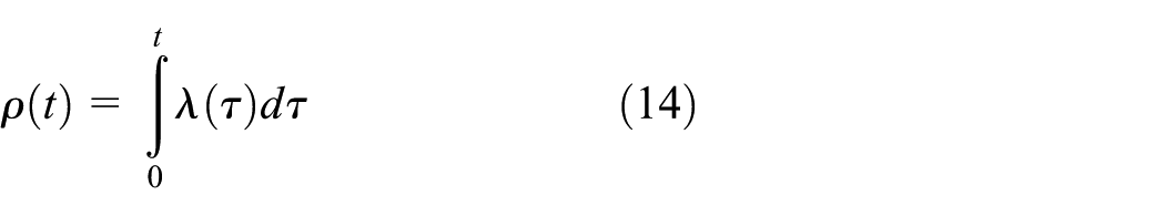
For the wear of SG tubes, the wear depth growth rate will change during the operation of nuclear power plants. In other words, the wear depth growth rate should be treated as a time-dependent variable, which is applied to evaluate the process intensity. Then, a non-homogeneous linear growth Markov process is assumed. The non-homogeneous linear growth Markov process is considered as a pure birth process with

λ_{i} (t) = i λ (t)

(12)

Here, the intensity $λ_{i} (t)$ is the number of transition states that the process leaves the state i over very short time. The function $λ (t)$ can be interpreted as the jump frequency of the wear depth that increases by one state during a very short interval of time h at t. In other words, the jump frequency can be regarded as a ratio of the number of transition states to i states over h at t. Then, $(d_{0} / N) λ (t)$ is related to the wear depth growth rate, where d₀ is the initial thickness.

The solution of Kolmogorov’s forward equation for the transition probability $p_{m, n} (t_{0}, t)$ from state m to state n in the interval $(t_{0}, t)$ can be obtained and has the form

p_{m, n} (t_{0}, t) = (\begin{matrix} n - 1 \\ n - m \end{matrix}) e^{- {ρ (t) - ρ (t_{0})} m} {(1 - e^{- {ρ (t) - ρ (t_{0})}})}^{n - m}

(13)

where

ρ (t) = \int_{0}^{t} λ (τ) d τ

(14)

In words, equation (13) means that the increase in the wear depth over $Δ t = t - t_{0}$ follows a negative binomial distribution NegBin(r, p) with parameter $r = m$ and $p = p_{s} = e^{- {ρ (t) - ρ (t_{0})}}$ . It should be noted that there is no upper limit for the state space in the pure birth process. To solve the problem, an absorbing state is considered when the wear depth reaches the thickness of the tube. According to the transition probability $p_{m, n} (t_{0}, t)$ , the probability density function (PDF) of the state growth rate v over the time interval $Δ t = t - t_{0}$ can be estimated as³¹

f (v; m, t_{0}, t) = p_{m} (t_{0}) p_{m, m + v Δ t} (t_{0}, t) Δ t

(15)

when the wear depth is at state m.

For all the possible states at t₀, the marginal distribution of the state growth rate v can be derived as

\begin{matrix} f (v; t_{0}, t) = \sum_{m = 1}^{N} f (v; m, t_{0}, t) \\ = \sum_{m = 1}^{N} p_{m} (t_{0}) p_{m, m + v Δ t} (t_{0}, t) Δ t \end{matrix}

(16)

Consider the wear depth is in state m at t₀. According to the negative binomial distribution NegBin(r, p_s) as equation (13), the expectation of state growth rate v over the time interval $Δ t = t - t_{0}$ can be obtained as

E (v; m, t_{0}, t) = \frac{E (n - m)}{Δ t} = \frac{m (1 - p_{s})}{p_{s} Δ t}

(17)

Parameter estimation

To sum up, the key of determining the wear depth distribution with time is the transition probability $p_{m, n} (t_{0}, t)$ , which depends on the jump frequency $λ (t)$ . If the jump frequency is determined, the wear depth can be predicted. Considering the measured data, the mean wear depth of the process can be obtained by eddy current inspection. It is postulated that the stochastic mean pit depth $M (t)$ is equal to the observed mean wear depth $H (t)$ as

M (t) = H (t)

(18)

If the initial damage state is $n_{i}$ at $t = t_{i}$ , so that $D (t_{i}) = n_{i}$ , then the time-dependent stochastic mean of the wear depth for the linear growth Markov process can be expressed as

M (t) = n_{i} e^{ρ (t - t_{i})}

(19)

If the first state is assumed to be 1 at the beginning of the power plant, so that $n_{i} = 1$ and $t_{i} = 0$ , the value of the function $ρ (t)$ can be approximated as

ρ (t) = \ln [H (t)]

(20)

From the equation above, considering equation (18), the jump frequency of the Markov process follows that

λ (t) = \frac{d \ln [H (t)]}{dt} = \frac{1}{H (t)} \frac{dH (t)}{dt}

(21)

Here, $dH (t) / dt$ can be regarded as the measured growth rate of wear depth which can be estimated on the ISI data.

Application and discussion

Data resource

To validate the proposed model for wear, the inspection records³² from SG tube inspection report for Point Beach Nuclear Plant Unit 1 are used in this study. Point Beach Unit 1 contains two Westinghouse Model 44F SGs, which were installed in 1983 to replace the original Unit 1 SGs. Until the inspection conducted in March 2016 during refueling outage U1R36, the Unit 1 SGs had accumulated 27.1 effective full power years (EFPYs) of operation. The inspection records listed the AVB wear indications and TSP wear indications identified in SG A with each indication’s historical depth measurements from 1995 (the 22nd refueling outage, U1R22).

To analyze the wear depth growth behavior, the inspection data screened out the new birth indications, and the selected data are shown in Figure 2, where %TW means the ratio of wear depth to the thickness of wall. There are total 34 locations where wear indications identified as shown in Figure 2(a) with different markers. They are monitored during every ISI from 1995 to 2016. In all, 306 indications of wear depth are obtained with nine data logs (nine ISI records) in each location. To show clearly, four typical locations are lined with neighboring ISI. It can be seen that there is obviously uncertainty in the measurement of wear depth at the same location. In addition, some wear indications show a reduced wear depth between the two adjacent refueling outages, which may be caused by the measurement error, inspection technology, human factor, and so on. However, the wear depth should be a monotonically non-decreasing function with time-dependence from a physical point of view. The mean of wear depth with SG operation is also plotted in Figure 2(b). It can be seen that there is limited increase in its mean. However, it shows an increased scatter, which can be found by the change of maximum and minimum.

Figure 2.

AVB wear indications in SG A: (a) all filtered indications and (b) mean, maximum, and minimum of wear depth.

Figure 3 shows the number of indications for each AVB wear depth in SG A during U1R22 in 1995. For the 34 indications, a lognormal distribution can fit them well with parameters μ = 2.0126 and σ = 0.5219, as shown in this figure for the PDF with

f (x, μ, σ) = \frac{1}{\sqrt{2 π} σ x} e^{[- \frac{1}{2} {(\frac{\ln x - μ}{σ})}^{2}]}

(22)

Figure 3.

AVB wear indications in SG A during U1R22 in 1995.

The other ISI records are also fitted by lognormal distribution, and the parameters are listed in Table 1.

Table 1.

Distribution parameters for the ISI data by lognormal distribution.

Date	2016	2013	2011	2008	2007	2004	2001	1998	1995
EFPY	27.1	24.3	22.9	20.1	18.7	16.0	13.2	10.6	8.7
M	2.5775	2.6214	2.5864	2.3627	2.5729	2.4257	2.3678	2.0931	2.0126
Σ	0.5037	0.4496	0.506	0.5043	0.3991	0.4748	0.5292	0.4039	0.5219

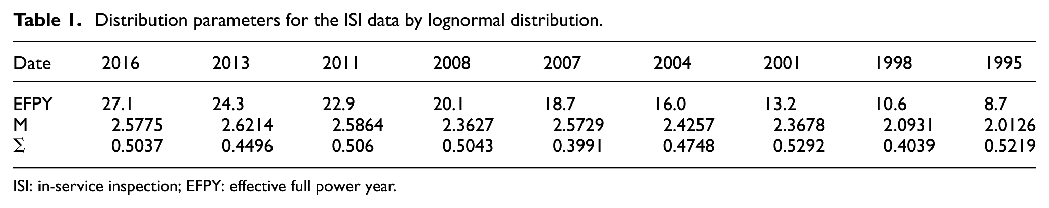
ISI: in-service inspection; EFPY: effective full power year.

To exam the transition intensity, the wear depth growth rates are evaluated. The average depth growth rates can also be estimated via the inspection data of the neighbor inspections. Figure 4 shows the empirical distribution function of the wear depth growth rate over 1.96 EFPY from 1995 to 1998, using Benard’s approximation equation

F = \frac{i - 0.3}{N + 0.4}

(23)

Figure 4.

Wear depth growth rate over 1.96 EFPY from 1995 to 1998.

From a physical point of view, the wear depth growth rate should not be negative. Not surprisingly, negative growth rates can be found from industry service experience, as shown in Figure 4. A negative tail of the measured growth rate distribution may be caused by the NDE sizing uncertainty. For a given location, the indication of wear depth identified at the current ISI may be lower than the indication identified at the previous time, as shown in Figure 2(a). This situation will show a negative growth rate. In general, the NDE sizing uncertainty will result in this situation, including measurement equipment, inspectors, size characterization, and so on. To obtain a conservative estimation, negative growth rates sometimes are set equal to zero. However, this will result in overly conservative growth rates. The estimates of the 50th and 95th percentiles of the measured distribution are about 0.51%TW/EFPY and 2.55%TW/EFPY, respectively, while the global average wear depth growth rate is about 0.16%TW/EFPY using all NDE-measured growth rate data including negative values. These estimates will be used to evaluate the transition intensity of the Markov model.

Wear depth distributions

The proposed continuous-time Markov chain model for wear is applied to estimate the distribution of wear depth for the future operation of SG. The ISI data during U1R22 in 1995 are employed. Then, the initial time t₀ equals to 8.7 EFPY. According to the analysis of data resource described in the above section, we can estimate the mean of wear depth by the growth rate. The mean of wear depth in the next inspection H(t) is about 9.41%TW over t–t₀ = 1.96 EFPY using the growth rate of v = 0.51%TW/EFPY with initial mean of 8.41%TW.

The wall thickness is divided into 100 discrete Markov states. According to equation (3), the wear depth distribution at the next inspection date t can be estimated as shown in Figure 5. In addition, the number of indications and fitted PDF are also plotted in this figure. It seems that the predicted distribution is almost the same as the fitted distribution. Besides, the Kolmogorov–Smirnov test is carried out to illustrate the goodness of fit by the comparison of the predicted distribution and empirical distribution. The Kolmogorov–Smirnov statistic is computed, D_n = 0.102. 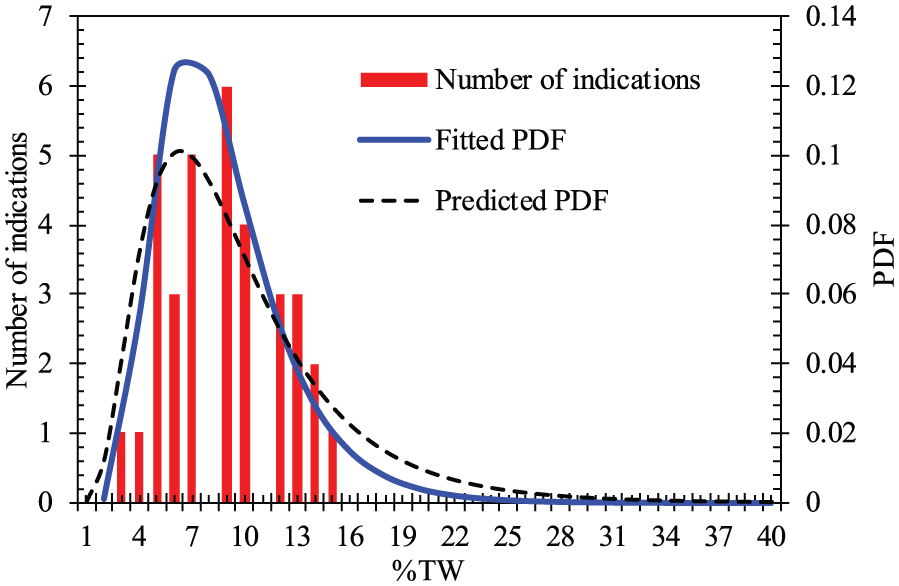It is lower than the critical values of the Kolmogorov distribution with a p-value of 0.995, $D_{34, 0.005} = 0.273$ . Therefore, the null hypothesis that the sample comes from the predicted distribution can be accepted.

Figure 5.

AVB wear indications during U1R24 in 1998.

Figure 6 shows the wear depth distributions predicted on the ISI data in 1995 for the future inspections. Using the ISI data, Kolmogorov–Smirnov tests are also performed to show that a p-value of 0.995 is enough to accept the null hypothesis. The results of Kolmogorov–Smirnov statistic are shown in Figure 7.

Figure 6.

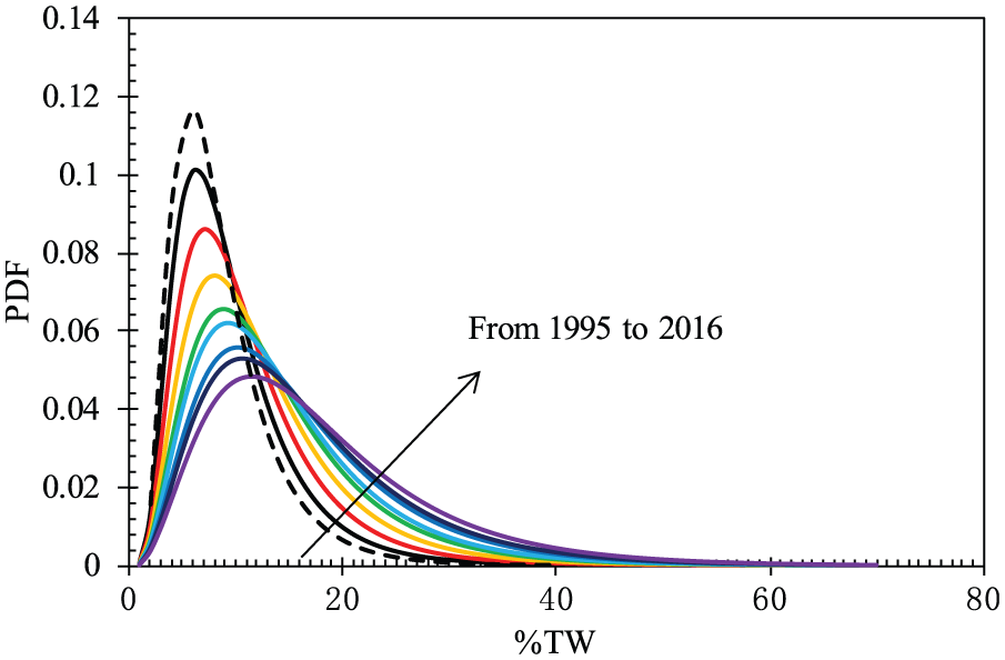
Wear depth distributions predicted on the ISI data in 1995.

Figure 7.

Kolmogorov-Smirnov statistics of the predicted wear depth on the ISI data in 1995.

Wear depth growth rate distribution

As mentioned above, the mean wear depth is necessary to determine the intensity of the Markov process as equation (21). In the above section, the average wear depth is calculated by an estimate of the 50th percentile of the measured growth rate distribution. It should be noted that the wear depth growth rate will have a significant effect on the predicted results. Therefore, the distribution of wear depth growth rate is discussed.

The predicted wear depth growth rate distribution is shown in Figure 8, which is calculated following equation (16) over the operation from 1995 to 1998. It should be noted that a negative growth rate is impossible in prediction model. However, it does exist in the measured ISI data because of the NDE sizing errors.¹² A recommended procedure is applied to distinguish best estimate actual growth rate distributions from NDE-measured growth rates using Monte Carlo simulation. Figure 8 shows a comparison with the estimated actual growth rate and the predicted growth rate using Markov Chain model in this work. For the distribution of growth rate, it can be seen that the predicted value comes closer to the NDE-measured value than the estimated value using Monte Carlo simulation. The reason for the error is that a negative growth rate is set to be zero with conservative consideration during the estimation using Monte Carlo simulation. The estimated actual growth rate distribution matches the NDE-measured growth rate distribution at the 50th percentile point, as shown in Figure 8. Compared with the estimated actual growth rate distribution, the predicted growth rate either at the 50th percentile point or the 95th percentile point is larger. Therefore, the wear depth estimated by the predicted growth rate should be conservative using the 50th percentile point or the 95th percentile point. Therefore, the predicted growth rate can be accepted for engineering practice.

Figure 8.

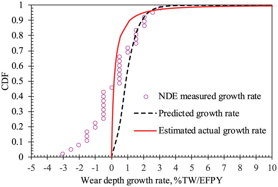
CDF of wear depth growth rate over 1.96 EFPY from 1995 to 1998.

The NDE-measured growth rate is analyzed using all growth rate data from 1995 to 2016. The estimates of the 50th percentile of the measured distribution are about 0.36%TW/EFPY, while the average is about 0.22%TW/EFPY. It can be seen that large growth rates incur at some locations with a maximum of 6.9%TW/EFPY and a minimum of –7.8%TW/EFPY. Obviously, the scatter is more serious than its estimation on the measured data from 1995 to 1998. Fortunately, the 50th percentile by the global data is similar to the one by local data set from 1995 to 1998. Therefore, the predicted wear depth can obtain a well agreement with the measured data, as shown in Figure 9.

Figure 9.

CDF of wear depth growth rate using the global data from 1995 to 2016.

Conclusion

A non-homogeneous Markov process model of wear is proposed to assess the evaluation of wear depth in SG tubes. The model is adopted for an SG operated from 1995 to 2016. Based on the results and discussions presented herein, the key findings of this study can be summarized as follows:

Based on the analytical solutions of the system of Kolmogorov’s forward equations, the transition probability functions were computed to estimate the future wear depth distribution. The parameters are estimated under the assumption that the mean wear depths in the proposed Markov stochastic model are equal to the average of measured depths.

The proposed Markov stochastic model was tested with ISI records according to a report for SG tube inspection from 1995 to 2016. The average measured depth and wear depth growth rate, drawn from the ISI data, are used to determine the initial parameters in Markov model.

The results showed a good agreement with future wear depth distribution. Compared with the empirical distributions, the predicted distribution can be accepted with 99.5% confidence by Kolmogorov–Smirnov test. The predicted growth rate either at the 50th percentile point or the 95th percentile point is larger than the estimated actual growth rate over the operation from 1995 to 1998. The global wear depth growth rate can also be predicted well.

It should be noted that the case data applied in this work are filtered just for the wear growth process, while the generation of new wear damage is not considered. However, new wear damage is excepted during the long operation, which can be also simulated by some stochastic processes, such as Poisson process. It should be further studied to combine these processes.

Footnotes

Acknowledgements

The authors acknowledge Dr Yi Liu for the suggestion on the Markov process and Dr Chen Chen for the preparation of the manuscript.

Handling Editor: James Baldwin

Declaration of conflicting interests

The author(s) declared no potential conflicts of interest with respect to the research, authorship, and/or publication of this article.

Funding

The author(s) disclosed receipt of the following financial support for the research, authorship, and/or publication of this article: This research was funded by the National Natural Science Foundation of China (grant nos 51605435 and 11602219), Zhejiang Provincial Natural Science Foundation of China (grant no. LQ16A020004); and National Key R&D Program of China (grant no. 2018YFC0808804).

ORCID iD

Yuebing Li

References

Guérout

Fisher

NJ.

Steam generator fretting-wear damage: a summary of recent findings. J Press Vess-T ASME 1999; 121: 304–310.

Diercks

Shack

Muscara

Overview of steam generator tube degradation and integrity issues. Nucl Eng Des 1999; 194: 19–30.

Auvinen

Jokiniemi

Lähde

et al . Steam generator tube rupture (SGTR) scenarios. Nucl Eng Des 2005; 235: 457–472.

Meng

Ludema

KC.

Wear models and predictive equations: their form and content. Wear 1995; 181: 443–457.

Au-Yang

MK.

Flow-induced wear in steam generator tubes—prediction versus operational experience. J Press Vess-T ASME 1998; 120: 138–143.

Fisher

Chow

Weckwerth

MK.

Experimental fretting-wear studies of steam generator materials. J Press Vess-T ASME 1995; 117: 312–320.

Lee

Kim

Kang

et al . A study on wear coefficients and mechanisms of steam generator tube materials. Wear 2001; 250: 718–725.

Yun

Lee

Hur

et al . Effect of oxidation film on the fretting wear behavior of Alloy 690 steam generator tube mated with SUS 409. Wear 2016; 368–369: 344–349.

Lai

Gao

Tang

et al . Effect of temperature on fretting wear behavior and mechanism of alloy 690 in water. Nucl Eng Des 2018; 327: 51–60.

10.

Amanov

Umarov

The effects of ultrasonic nanocrystal surface modification temperature on the mechanical properties and fretting wear resistance of Inconel 690 alloy. Appl Surf Sci 2018; 441: 515–529.

11.

Attia

Magel

Experimental investigation of long-term fretting wear of multi-span steam generator tubes with U-bend sections. Wear 1999; 225–229: 563–574.

12.

Electric Power Research Institute. Steam generator integrity assessment guidelines (Revision 2), Report no. EPRI 1012987, July 2006. Palo Alto, CA: Electric Power Research Institute.

13.

Ferng

Fan

Pei

et al . Predicting the accumulated number of plugged tubes in a steam generator using statistical methodologies. Ann Nucl Energy 2008; 35: 1912–1918.

14.

Ferng

YM.

Predicting growth rate of wall thinning for severely degraded SG tubes using a statistical methodology. Nucl Eng Des 2010; 240: 129–131.

15.

Xie

Stochastic modelling and analysis of degradation for highly reliable products. Appl Stoch Models Bus Ind 2015; 31: 16–32.

16.

Whitmore

Schenkelberg

Modelling accelerated degradation data using wiener diffusion with a time scale transformation. Lifetime Data Anal 1997; 3: 27–45.

17.

Park

Padgett

WJ.

Accelerated degradation models for failure based on geometric Brownian motion and gamma processes. Lifetime Data Anal 2005; 11: 511–527.

18.

Doksum

Hóyland

Models for variable-stress accelerated life testing experiments based on wiener processes and the inverse Gaussian distribution. Technometrics 1992; 34: 74–82.

19.

Wang

Tsui

KL.

Stochastic evaluation of magnetic head wears in hard disk drives. IEEE Trans Magn 2014; 50: 1–7.

20.

Kharoufeh

JP.

Explicit results for wear processes in a Markovian environment. Oper Res Lett 2003; 31: 237–244.

21.

Liang

Tang

et al . A weighted hidden Markov model approach for continuous-state tool wear monitoring and tool life prediction. Int J Adv Manuf Tech 2017; 91: 201–211.

22.

EM Li

Jiang

et al . An optimal reprofiling policy for high-speed train wheels subject to wear and external shocks using a semi-Markov decision process. IEEE Trans Reliab 2018; 67: 1–14.

23.

Zhu

Liu

Online tool wear monitoring via hidden semi-Markov model with dependent durations. IEEE Trans Ind Inf 2018; 14: 69–78.

24.

Valor

Caleyo

Alfonso

et al . Stochastic modeling of pitting corrosion: a new model for initiation and growth of multiple corrosion pits. Corr Sci 2007; 49: 559–579.

25.

Caleyo

Velázquez

Valor

et al . Markov chain modelling of pitting corrosion in underground pipelines. Corr Sci 2009; 51: 2197–2207.

26.

Valor

Caleyo

Alfonso

et al . Markov chain models for the stochastic modeling of pitting corrosion. Math Probl Eng 2013; 2013: 1–13.

27.

Zhu

Huang

Smith

et al . Bayesian framework for probabilistic low cycle fatigue life prediction and uncertainty modeling of aircraft turbine disk alloys. Probab Eng Eng Mech 2013; 34: 114–122.

28.

Zhu

Huang

Peng

et al . Probabilistic physics of failure-based framework for fatigue life prediction of aircraft gas turbine discs under uncertainty. Reliab Eng Syst Saf 2016; 146: 1–12.

29.

Xie

Zhang

Aldemir

et al . Multi-state Markov modeling of pitting corrosion in stainless steel exposed to chloride-containing environment. Reliab Eng Syst Saf 2018; 172: 239–248.

30.

Parzen

Stochastic processes. Philadelphia, PA: SIAM, 1999.

31.

Ossai

Boswell

Davies

Markov chain modelling for time evolution of internal pitting corrosion distribution of oil and gas pipelines. Eng Fail Anal 2016; 60: 209–228.

32.

NextEra Energy Point Beach, LLC. Spring 2016 unit 1 (U1 R36) steam generator tube inspection report. Report no. ML16264A202, 20 September 2016. Washington, DC: Nuclear Regulatory Commission.

Markov stochastic process modeling for evolution of wear depth in steam generator tubes

Abstract

Keywords

Introduction

Markov stochastic process model of wear

Continuous-time Markov chain model

Transition probability

Parameter estimation

Application and discussion

Data resource

Wear depth distributions

Wear depth growth rate distribution

Conclusion

Footnotes

Acknowledgements

Declaration of conflicting interests

Funding

ORCID iD

References