A new integrated numerical modeling approach toward piston diaphragm pump simulation: Three-dimensional model simplification and characteristic analysis

Abstract

Piston diaphragm pumps are used worldwide to transport abrasive and aggressive slurries against high discharge pressures in the mining, mineral processing, and power industries. Intermittent suction and drainage of the diaphragm, however, can lead to pulsating output pressure, which has caused major problems in the application of these pumps. To improve the accuracy of simulations of piston diaphragm pumps and to enable better simulation of their pressure pulsation behavior, it is necessary to carry out a three-dimensional fluid–structure interaction simulation of the pump fluctuation characteristics. This article proposes a simplified simulation model based on the periodic motion characteristics of a piston diaphragm pump, where a ZMB240 piston diaphragm pump serves as the research object. By simplifying the numerical simulation of the model, we are able to analyze the deformation characteristics and the fluctuation characteristics of the piston diaphragm pump under different initial conditions for the pressure-stabilizing air chamber.

Introduction

Introduction to the piston diaphragm pump

Piston diaphragm pumps are widely used in the mining, mineral processing, and power industries to transport abrasive and aggressive slurries against high discharge pressures. ¹ However, the complex internal flow of a piston diaphragm pump can generate hydraulic excitation forces that cause pressure pulsations. ² Figure 1 shows the structure of a ZMB240 piston diaphragm pump. This pump consists of a pump body, a side cover, a diaphragm, inlet and outlet valves, an eccentric shaft, a piston, a slider, and an air chamber. When the eccentric shaft rotates, the piston is then driven to reciprocate by the slider. When the piston moves from top dead center to bottom dead center, a vacuum is formed between the top surface of the piston and the diaphragm. The diaphragm then deforms in the direction of the bottom dead center position of the piston, thus causing a vacuum between the side cover and the diaphragm. At this point, the liquid outside the pump enters the pump chamber through the inlet pipe under the action of atmospheric pressure until the piston moves to bottom dead center and the pump chamber then completes the pipetting process.

Figure 1.

Structure of piston diaphragm pump.

The construction and functions of the main components of the piston diaphragm pump are described as follows:

1. Pump body: The body forms the basis of the pump and contains a piston cylinder hole, a bearing hole, and a water inlet. The pump body and the diaphragm constitute the pump room.

2. Side cover: This covers the pump and is installed on both sides of the pump body.

3. Diaphragm: The diaphragm is bowl shaped and is used for energy conversion.

4. Inlet and outlet valves: These valves have identical structures and are each composed of a valve seat, a valve cover, and a valve body bracket; however, they have different installation positions.

5. Air chamber: This chamber is used to stabilize the working pressure of the pump and consists mainly of an air chamber seat, an air chamber cover, and the diaphragm. The chamber separates the air into upper and lower parts. The upper part is inflated, while the lower part takes on liquid.

During operation of the ZMB240 piston diaphragm pump, the intermittent suction and discharge action of the diaphragm pump causes deformation of the rubber diaphragm, which results in changes in the gas and liquid domains inside the pump. Therefore, the fluid-diaphragm-compressed air configuration has fluid–structure interaction (FSI). The FSI fluid–solid coupling module can perform bidirectional fluid–solid coupling simulations of the three-dimensional (3D) model of the diaphragm pump’s liquid, gas, and rubber diaphragm to obtain the dynamic deformation characteristics of the diaphragm.

FSI application

FSI, which can lead to increased potential for flow-induced vibration, structural wear and even structural failure under worst-case conditions, occurs between the complex internal flow and the structures of a piston diaphragm pump. ² FSI is a natural phenomenon that was first recognized in studies of aeroelastic problems in the early 19th century. Zienkiewicz and Taylor ³ defined FSI as a coupled system. FSI formulations apply to multiple domains and dependent variables that usually describe different physical phenomena; in these formulations, neither domain can be solved separately from its counterpart and neither of the sets of dependent variables can be explicitly eliminated at the different equation levels. There is a growing body of literature with regard to FSI in turbomachinery, with several studies of turbines,^4–6 while a few have discussed pumps. Pei et al. ⁷ investigated the flow-induced vibrations of a commercial single-blade sewage water pump using both numerical and experimental methods. They concluded that it is possible to determine the rotor oscillations using numerical codes for the transient flow in the pump and the structural dynamics of the rotor. Wang et al. ⁸ predicted the noise from a multistage centrifugal pump using a one-way coupling method. Langthjem and Olhoff ⁹ investigated the flow-induced noise in a two-dimensional centrifugal pump and found that the interaction between the fluid and the rotating impeller blades plays an important role in noise generation.

Contributions of this study

The research described above indicates that FSI is a relatively mature subject in mechanical dynamics research, but no specific research has been conducted to date on the piston diaphragm pump. To improve the accuracy of the simulations of this type of pump and to simulate its pressure pulsation behavior, a 3D FSI simulation of the fluctuation characteristics of a diaphragm pump is required. A piston diaphragm pump consists of a diaphragm, a piston, a pump shaft, and several other complex components. However, importing the entire 3D structure of a diaphragm pump into ANSYS simulation software (Canonsburg, PA, USA) will greatly increase the difficulty and the computational cost of such an FSI simulation.

This article proposes a simplified simulation model based on the periodic motion characteristics of the diaphragm pump, with a ZMB240 piston diaphragm pump acting as the research object. By simplifying the numerical simulation of the model, we are able to analyze the deformation characteristics and the fluctuation characteristics of the piston diaphragm pump under different initial conditions for the pressure-stabilizing air chamber.

Model simplification

A 3D model of a ZMB240 piston diaphragm pump is shown in Figure 2. To show the internal structure clearly, two cross-sectional views of the diaphragm pump are provided. The various components of the pump body are made from gray cast iron. The material is HT200 cast iron and its hardness is HB143-269. The weight of the blank is approximately 2 kg. The manufacturing accuracy for each pump element is 0.1 mm. The rubber diaphragm used in the pump is made from fluororubber, which has the following characteristics. (1) To provide a reliable seal at the fixed diaphragm, the rubber material has a good stress relaxation value when used over long time periods. (2) Under a given pressure, the rubber offers sufficient strength, elasticity, notch impact resistance and wear resistance. Material fatigue does not occur under dynamic load conditions. (3) The rubber has good fluidity. (4) The material does not break as a result of changes in the climatic conditions and maintains sufficient elasticity at the lowest operating temperature. The most prominent feature of the ZMB240 piston diaphragm pump is its pressure-stabilizing air chamber, which is used to buffer the output pressure fluctuations of the diaphragm pump. To illustrate the main components of the diaphragm pump more clearly, the main pump components are drawn separately in three dimensions, as shown in Figure 3.

Figure 2.

ZMB240 piston diaphragm pump. 1. Pressure-stabilizing air chamber; 2. Outlet; 3. Side cover; 4. Inlet; 5. Pump shaft and slider assembly; 6. Pump body; 7. Air chamber diaphragm; 8. Working diaphragm.

Figure 3.

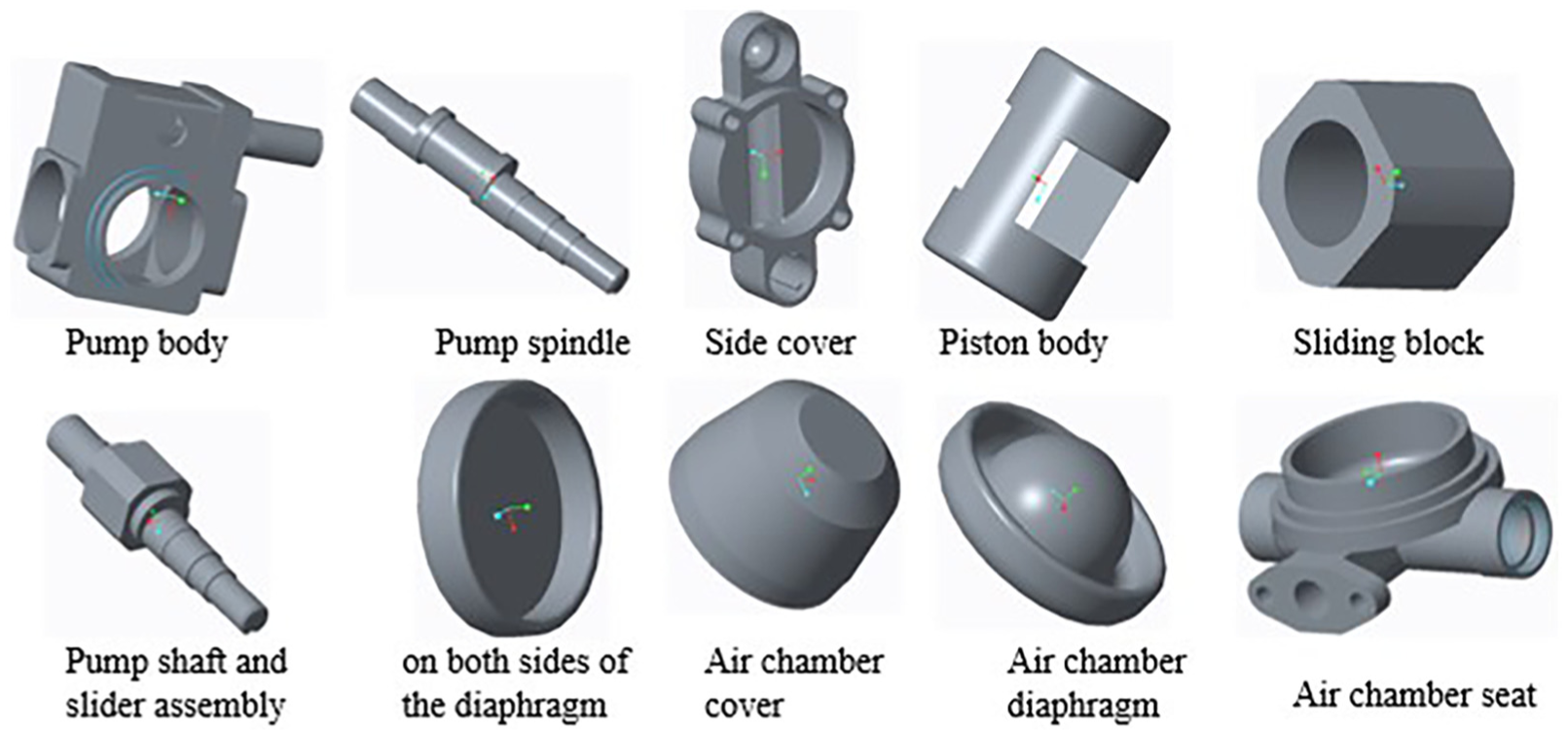
Three-dimensional views of the diaphragm pump’s main components.

Simplification of the diaphragm pump

Depending on the periodic motion of the diaphragm pump, the diaphragm agitation shaft on both sides of the pump has intermittent liquid suction and discharge characteristics. The complex components of the diaphragm pump make it difficult to use the entire diaphragm geometry as a computational fluid dynamics (CFD) analysis model when modeling the 3D flow path. In addition, the complexity of such a 3D model greatly increases the number of fluid meshes required, thus increasing the computational cost. The complex dynamic grid required for the pump shaft will also increase the difficulty of fluid–solid coupling simulations. To reflect the pressure fluctuation characteristics of the diaphragm pump accurately, we have simplified the diaphragm pump model.

The simplified model is illustrated in Figure 4. It is most important to obtain a function expression for the speed at both inlet sides of the diaphragm pump, which can simplify the check valves on both sides of the diaphragm, the pump shaft, the slider, and other pump components. The essential aim of a 3D dynamic simulation of the diaphragm pump is to study the pressure fluctuations caused by the periodic suction and drainage behavior, so the simplification of the speed inlet function does not affect the simulation results for the diaphragm pump. The most prominent feature of the ZMB240 piston diaphragm pump is its pressure-stabilizing air chamber. This air chamber and the rubber diaphragm are the most important research objects that are retained in the simplified model.

Figure 4.

Simplified diaphragm pump model.

Adams analysis of slider mechanism of pump shaft

We imported the pump shaft and slider assembly drawings into Adams multibody dynamics simulation software, to which we also added the kinematic pair and the drive for the simulation model.

1. Added kinematic pair: We arranged the rotating pairs between the sliding block and the pump shaft and between the pump shaft and the ground. The sliding block of the diaphragm pump does not exist in the axial direction during actual movement, so we established a plane restraint between the sliding block and the vertical plane.

2. Added drive: Based on the rated speed of the diaphragm pump, given by n = 600 r/min, we applied a speed of 3600 d/s to the pump shaft with a cycle time of T = 0.1 s.

In the Adams software, the default unit is d/s, which represents the angular distance per second. Therefore, we converted 600 r/min into 600 × 360/60 d/s = 3600 d/s.

Slider stroke motion function fitting

We used Origin data-processing software to fit the stroke motion function of the slider. We imported the stroke data of a slider in a single cycle from Adams into the Origin software. We estimated the function using the data graph as a nonstandard normal function; x is defined as the stroke of the slider in this case. Given the parameters, the function type selected the normal function for fitting using the following fitting equation

$$x=-1.24+5.68e^{-100{(t-0.05)}^2}(0\le t\le 0.1\mathrm{s})$$

Simplification of diaphragm motion on both sides of diaphragm pump

The operating principle of the ZMB240 piston diaphragm pump is known. The intermittent suction and discharge action of the diaphragm pump causes the volume deformation of the diaphragm on both sides of the pump. The deformation of the two sides of the diaphragm caused by the movement of the slide block is complex. To determine the change in volume of the diaphragm cavity caused by the deformation of the diaphragm, we first supposed that the diaphragm has a spherical cap shape, for which a deformation diagram is shown in Figure 5. The solid circle represents the deformation before the diaphragm pump action. The rough dashed line represents the subsequent deformation of the diaphragm. The fine dotted line indicates the auxiliary line. In Figure 5, a denotes the radius of the diaphragm before deformation, b denotes the displacement of the center caused by the deformation of the diaphragm, and R denotes the radius of the deformed ball. $\xi$ is defined as the correction factor with respect to the amount of volume change before and after deformation of the diaphragm.

Figure 5.

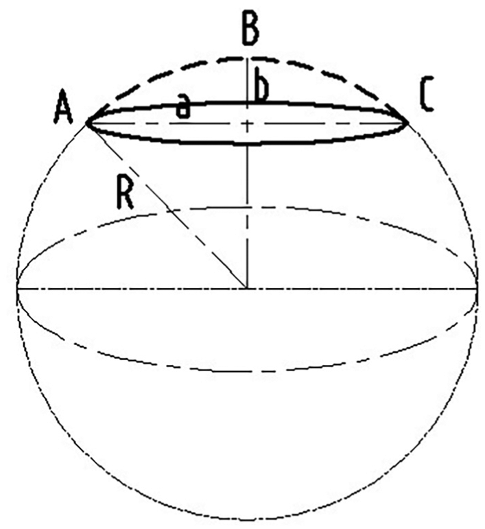
Diaphragm deformation diagram.

From the geometric relationship $(R-b{)}^2+a^2=R^2$ , we obtain

$$R=\frac{a^2+b^2}{2b}$$

(1)

The formula for the deformation volume of the diaphragm is

$$Q=\frac{\pi }{3}\xi (3R-b)*b^2$$

(2)

The speed formula in hydrodynamics is

$$V=\frac{\mathrm{dQ}}{\mathrm{dt}*A}$$

(3)

where Q is the flow and A is the cross-sectional area of the pipe. The pipe’s cross-sectional area is given by

$$A=\frac{\pi D^2}{4}$$

(4)

From equations (1)–(4), we obtain the following speed formula:

$$V=0.00154*\stackrel{.}{\xi *b}(9025+b^2)$$

(5)

The solution for the expected value E(X) is given by

$$E(X)=\underset{-\infty }{\overset{+\infty }{\int }}\mathrm{xf}(x)\mathrm{dx}$$

(6)

We thus obtain $\xi \approx 0.0123$

$$V=1.9*(9025+b^2)b*10e^{-5}$$

(7)

$$b=-1.24+5.68e^{-100{(t-0.05)}^2}(0\le t\le 0.1\mathrm{s})$$

(8)

Establishment of simplified model of diaphragm pump

Before the numerical simulation could be performed, the simulation model for the diaphragm pump fluid domain had to be built. For this work, we realized a 3D flow passage extraction model of the diaphragm pump using the ANSYS Workbench geometry module. We then obtained a fluid-flow simulation model of the ZMB240 piston diaphragm pump, as illustrated in Figure 6(a); the model of the elastic element is shown in Figure 6(b).

Figure 6.

Simulation model: (a) fluid-flow simulation model of the ZMB240 piston diaphragm pump and (b) model of the elastic element.

We assembled the fluid–solid coupling simulation model of the ZMB240 piston diaphragm pump with the gas domain model and the rubber diaphragm solid model using 3D drawing software to obtain the final Workbench simulation model. The four monitoring points in the model are labeled in Figure 7.

Figure 7.

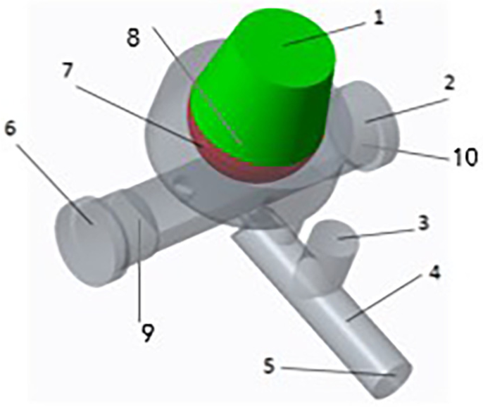
Diaphragm pump simulation model. 1. Air chamber gas domain model; 2. Right speed inlet; 3. Overflow outlet; 4. Outlet pressure monitoring point; 5. Diaphragm pump outlet; 6. Left speed inlet; 7. Diaphragm solid domain model; 8. Gas (air) pressure monitoring point; 9. Left inlet pressure monitoring point; 10. Right inlet pressure monitoring point.

Numerical simulation

Methodology

The simulation was performed based on the Reynolds-averaged Navier–Stokes (RANS) equations and a standard steady-state k–ε turbulence model. The governing equations are as shown below. The continuity equation in incompressible form ¹⁰ is

$$\frac{\partial u_j}{\partial x_j}=0$$

(9)

and the Navier–Stokes equation is

$$u_j\frac{\partial u_i}{\partial x_j}=-\frac{1}{\rho }\frac{\partial p}{\partial x_i}+\frac{\mu }{\rho }\frac{{\partial }^2{u}_i}{\partial x_j\partial x_j}-\frac{\partial }{\partial x_j}(\overline{{u\prime }_i{u\prime }_j})+g_i$$

(10)

where g_i is the gravitational body force (g_i = −gδ_i3) and $-(\overline{{u\prime }_i{u\prime }_j})$ is the Reynolds stress, which is computed by relating the Reynolds stresses to the mean velocity gradients as follows:

$$-(\overline{{u\prime }_i{u\prime }_j})=\frac{1}{\rho }{\mu }_t(\frac{\partial u_i}{\partial x_j}+\frac{\partial u_j}{\partial x_j})-\frac{2}{3}k{\delta }_{\mathrm{ij}}$$

(11)

The turbulence closure equations for the turbulent kinetic energy k and the dissipation rate of the turbulent kinetic energy ε are given as equations (12) and (13), respectively:

$$u_j\frac{\partial k}{\partial x_j}=\frac{1}{\rho }\frac{\partial }{\partial x_j}\left[(\mu +\frac{{\mu }_t}{\sigma k})\frac{\partial k}{\partial x_j}\right]+\frac{G_k}{\rho }-\epsilon$$

(12)

$$u_j\frac{\partial \epsilon }{\partial x_j}=\frac{1}{\rho }\frac{\partial }{\partial x_j}\left[(\mu +\frac{{\mu }_t}{{\sigma }_{\epsilon }})\frac{\partial \epsilon }{\partial x_j}\right]+\frac{1}{\rho }{C}_{\epsilon 1}{G}_k\frac{\epsilon }{K}-C_{\epsilon 2}\frac{{\epsilon }^2}{K}$$

(13)

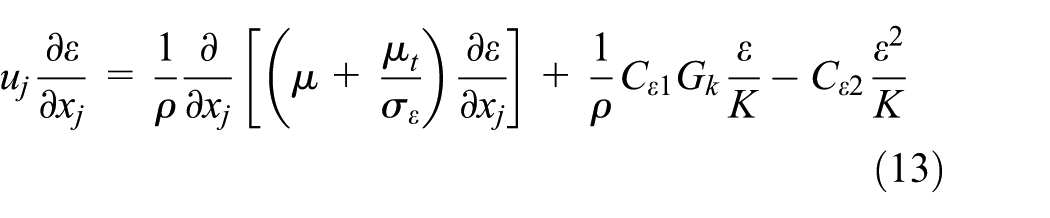
where µ is the dynamic viscosity, µ_t is the turbulent viscosity, and G_k is the turbulent kinetic energy production term.

Calculation model

Meshing

Because the fluid domain has an irregular shape, we used adaptive meshing in this calculation model. We controlled the unit size by setting the relevance value (the method can control the grid size automatically based on the characteristics of the physics field and the relevance value). To ensure calculation accuracy, the relevance value was set at 50. The FSI interface between the diaphragm and fluid domain used the same size for the grid scale to ensure both accurate transfer and the convergence of the calculated results for the flow field and the structure field. A tetrahedron grid cell was used and grid encryption was performed for the interaction between the fluid domain and the structure. The interface between the grid encryption processing stage and the relevant part of the grid produced poor quality results and it was necessary to apply a smoothing process. We used 3,804,786 grid cells for the flow field calculation and 69,852 grid cells for the rubber diaphragm.

Boundary conditions

Because the suction and discharge actions of the one-way valves on both sides of the diaphragm pump are intermittent, during the time interval of 0–0.05 s, the right check valve is open while the left check valve is closed; then, during the time interval of 0.05–0.1 s, the right check valve is closed while the left check valve is open. We calculated the fluid fluctuation characteristics of the diaphragm pump to obtain the stress and deformation characteristics of the diaphragm during pump operation. The diaphragm pump inlet was defined as the speed inlet and the interface between the liquid domain and the rubber diaphragm is defined as the water–solid wall. The air–solid wall is arranged at the interface between the gas domain and the rubber diaphragm. The upper surface of the solid domain is a solid–air wall. The lower surface is set as a solid–water wall.

Parameter settings

The Reynolds number is defined as

$$\mathrm{Re}=\frac{\rho \mathrm{vd}}{\mu }$$

where $\rho$ is the fluid density, $v$ is the average flow rate, $d$ is the pipe diameter, and $\mu$ is the dynamic viscosity coefficient. The average flow rate is $v=Q/A$ , where $Q$ is the flow. The Re was greater than 3000, which indicates that the fluid inside the diaphragm pump was in a turbulent state.

While the standard $k-\epsilon$ model is only suitable for the simulation of a full turbulent flow process, the renormalization group $k-\epsilon$ model is more suitable for the high-Reynolds-number flow problem, and the $k-\epsilon$ model can be implemented for a wide range of motion types. Therefore, the dynamic process in the solenoid valve action process system is modeled. In the simulation analysis, the $k-\epsilon$ model can be selected and the transport equations for $k$ and $\epsilon$ are

$$\{\begin{array}{c}\rho \frac{\mathrm{dk}}{\mathrm{dt}}=\frac{\partial }{\partial x}\left[(\mu +\frac{{\mu }_t}{{\sigma }_{\epsilon }})\frac{\partial \epsilon }{\partial x_i}\right]+G_k+G_b-\rho \epsilon -Y_M\hfill \\ \rho \frac{d\epsilon }{\mathrm{dt}}=\frac{\partial }{\partial x_i}\left[(\mu +\frac{{\mu }_t}{{\sigma }_{\epsilon }})\frac{\partial \epsilon }{\partial x_i}\right]+\rho C_{1}S\epsilon -\rho C_2\frac{{\epsilon }^2}{k+\sqrt{v\epsilon }}+C_{1\epsilon }\frac{\epsilon }{k}{C}_{3\epsilon }{G}_b\hfill \end{array}$$

where $C_1=max[0.43,\eta /(\eta +5)]$ , $\eta =\mathrm{Sk}/\epsilon$ , and $G_k$ is the turbulent energy caused by the average velocity gradient; $G_b$ is the turbulent energy caused by buoyancy; $Y_M$ represents the effect of compressible turbulent pulsation expansion on the total dissipation rate; ${\sigma }_k$ is the Prandtl number of the turbulent energy; ${\sigma }_{\epsilon }$ is the Prandtl number of the energy dissipation rate; $C_{1\epsilon }$ and $C_2$ are constants; and ${\sigma }_k$ and ${\sigma }_{\epsilon }$ are used as the default constants in Fluent CFD software.

The equation for the turbulence intensity is

$$I=0.16\ast {\mathrm{Re}}^{-1/8}=2\%$$

Using this theoretical analysis as a basis, the settings for the simulation were as selected as follows.

The airflow field simulation model is a turbulence model. The turbulence intensity is the most important feature that is used to describe the characteristics of the turbulent motion. Therefore, the turbulent motion characteristics at the inlet are usually characterized by the turbulence intensity, while the turbulent motion characteristics at the outlet are characterized by the backflow turbulence intensity. The inlet adopts the velocity inlet boundary conditions; the turbulence intensity is 2% and the hydraulic diameter is 30 mm. The diaphragm pump outlet is set as the pressure outlet. The backflow turbulence intensity is 2% and the hydraulic diameter of the backflow is 20 mm. We selected air as the gas domain material, set the initial pressure and the initial air chamber temperature, and finally selected water as the liquid domain material. Using a split solver, we selected the coupling velocity pressure method as the coupling method and used the second-order windward method to solve the problem. The related dynamic mesh settings were set with the water–solid wall and the air–solid wall acting as the coupling surfaces. We used the transient calculation model to set the number of iterations to 500 and the time step to 0.0001.

Results and discussion

Piston diaphragm pump deformation characteristic analysis under different initial pressures

In the simulation calculations, we set the initial pressure of the piston diaphragm pump pressure-stabilizing air chamber in the 0.3–0.7 MPa range. After the simulation is complete, the deformation data within the time range from 0.01 to 0.05 s are obtained. The results are shown in Figure 8.

Figure 8.

Diaphragm deformation characteristics under different pressure-stabilizing air chamber initial pressure conditions.

Figure 8 shows that the deformation of the diaphragm decreases as the initial pressure of the pressure-stabilizing air chamber increases. When x = 7 cm, the largest deformation can be obtained. The diaphragm deformation in actual practice remained consistent.

We extracted the initial displacement of the pressure-stabilizing air chamber at 0.3, 0.4, 0.5, 0.6, and 0.7 MPa under various conditions for the diaphragm maximum displacement data at each moment, as shown in Figure 9.

Figure 9.

Diaphragm maximum deformation trend chart for the 0–0.05 s period.

Figure 9 shows that the maximum deformation of the diaphragm initially increased and then decreased for a fixed initial pressure value, while the diaphragm deformation reached a maximum at time t = 0.0318 s. The maximum deformation at the bottom of the diaphragm under each condition is shown in Table 1.

Table 1.

Maximum diaphragm deformation under various conditions.

Initial pressure (MPa)	Maximum deformation (mm)
0.3	50.8
0.4	43.8
0.5	35.8
0.6	29.8
0.7	25.8

The results in Table 1 show that as the initial pressure of the pressure-stabilizing air chamber increased, the maximum diaphragm deformation decreased accordingly. During the actual working process of the piston diaphragm pump, as the pressure in the pressure-stabilizing air chamber increased, the difference between the diaphragm pump working pressure and the pressure in the pressure-stabilizing air chamber decreased. Therefore, the diaphragm deformation was indeed reduced. However, the initial pressure of the pressure-stabilizing air chamber is an important parameter for suppression of the output pressure pulsation from the piston diaphragm pump. Therefore, the initial pressure of the pressure-stabilizing air chamber cannot be too low. The deformation of the pressure-stabilizing air chamber diaphragm obtained in this work can act as a reference value for optimization of the working parameters of the piston diaphragm pump.

Piston diaphragm pump fluctuation characteristic analysis under various initial pressures in the pressure-stabilizing air chamber

The diaphragm pump outlet pressure characteristics at various times for initial pressure values of 0.3, 0.4, 0.5, 0.6 and 0.7 MPa in the pressure-stabilizing air chamber are shown in Figure 10.

Figure 10.

Outlet pressure under different pressure-stabilizing air chamber initial pressures of (a) P = 0.3 MPa, (b) P = 0.4 MPa, (c) P = 0.5 MPa, (d) P = 0.6 MPa and (e) P = 0.7 MPa.

The simulation results show that the intermittent movement of the diaphragm pump leads to the development of a pressure pulse at the diaphragm pump outlet. During the period from 0 to 0.05 s, the outlet pressure first increased and then decreased. The simulation data show that the average outlet pressure value of the diaphragm pump is independent of the initial pressure P of the pressure-stabilizing chamber. When the diaphragm pump pressure is 0.5 MPa, the average outlet pressure value fluctuates around 0.5 MPa. In addition, the outlet pressure oscillations occur near t = 0.05 s because at 0.05 s, the one-way valve at the left of the diaphragm closes while the one-way valve on the right opens at this time on the coupling, in line with the actual operation.

Experimental verification

We performed practical testing of diaphragm pumps using a test system. This test system is shown in Figure 11. The initial pressures of the piston diaphragm pump pressure-stabilizing air chamber were set at 0.3, 0.4, 0.5, 0.6, and 0.7 MPa. We used the initial pressure in the air chamber at the noted outlet pressures at various times to draw the curve shown in Figure 12. Table 2 lists the simulation data and the test data.

Figure 11.

Diaphragm pump test system. 1. Constant pressure tube; 2. Pressure sensor; 3. Electromagnetic valve; 4. Nozzle; 5. Nozzle; 6. Nozzle; 7. Nozzle; 8. Flow sensor.

Figure 12.

Measured outlet pressure values at initial pressure-stabilizing air chamber pressures of: (a) P = 0.3 MPa, (b) P = 0.4 MPa, (c) P = 0.5 MPa, (d) P = 0.6 MPa, and (e) P = 0.7 MPa.

Table 2.

Simulation data and test data.

Initial pressure P (MPa)	Minimum pressure: simulated value (MPa)	Minimum pressure: measured value (MPa)	Maximum pressure: simulated value (MPa)	Maximum pressure: measured value (MPa)	Average pressure: simulated value (MPa)	Average pressure: measured value (MPa)
0.3	0.38	0.35	0.71	0.64	0.511	0.495
0.4	0.42	0.48	0.657	0.65	0.503	0.536
0.5	0.465	0.46	0.612	0.64	0.508	0.536
0.6	0.385	0.39	0.642	0.57	0.513	0.493
0.7	0.445	0.51	0.732	0.7	0.515	0.525

As shown in Figure 12, the test results and the simulation results show the same trends. During the period from 0 to 0.05 s, the outlet pressure initially increased and then decreased. At the same time, as Table 2 shows, there is a small degree of error between the simulated and measured values. Because the actual tests were subject to numerous environmental factors, a certain error range is allowed between the measured and simulated values. Figure 12 and Table 2 demonstrate the reliability of the proposed simulation model. From the simulation results and analysis of the test results, we can conclude that the average pressure at the piston diaphragm pump outlet is independent of the initial pressure in the pressure-stabilizing air chamber.

Conclusion

In this article, we used a ZMB240 piston diaphragm pump as the research object. Based on the periodic motion of this diaphragm pump, we proposed a simplified method for development of the CFD simulation model. We studied the deformation characteristics of the gas chamber diaphragm and obtained the deformation results for the gas chamber diaphragm in a single cycle. We also studied the pressure fluctuation characteristics of the regulator chamber. Our findings were as follows.

1. The simplified CFD numerical simulation results for the ZMB240 piston-type diaphragm pump and the trends shown in the test results were basically consistent. The errors between the test values and the simulated values remained within an allowable range. This verified the reliability of the simulation model.

2. During operation of the diaphragm pump, as the initial pressure in the pressure-stabilizing air chamber increased, the deformation of the diaphragm decreased and the maximum deformation occurred at the top of the diaphragm. Under actual engineering conditions, the initial pressure of the pressure-stabilizing air chamber can be increased appropriately to reduce the deformation of the diaphragm.

On the basis of these findings, this study of the deformation characteristics of the air chamber diaphragm has demonstrated its significance.