Sage Journals: Discover world-class research

Abstract

By means of numerical simulation and experimental verification, this article investigates the hydraulic performance and pressure fluctuation of a tank-style axial-flow pump device. With orthogonal test, 16 schemes are designed concerning the different flow conditions of the inlet and outlet passages, and simulated calculations are done; then the non-steady numerical simulation of pressure fluctuation is carried out for the optimized pump device; a model test finally verifies the reliability of the simulated numerical values of the optimized scheme. The results show that using the orthogonal test, an optimized scheme of the inlet and outlet passages can be obtained; compared with the initial scheme, the optimized one reduces the hydraulic loss by 1.3 cm in the inlet passage and 7.96 cm in the outlet passage; numerical simulation witnesses the highest pump operating efficiency of 70.04%, efficiency of 66.82% with the design head of 1.36 m, and the corresponding flow of 34.31 m³/s; the model test verifies all the simulated values of the optimized scheme with the highest pump operating efficiency reaching 71.5% and the test efficiency arriving at about 64% when the design head is 1.36 m. Meanwhile, the highest pressure fluctuation appears at the entrance of the impeller; the main frequency of the impeller and guide vane pressure fluctuation is 5 Hz depending on the frequency of the blade. This study offers reference for similar pump station project.

Keywords

Tank-style pump device orthogonal test numerical simulation pressure fluctuation model test

Introduction

Bidirectional flow pump device, that is, tank-style pump device, can effectively achieve the purpose of irrigation and drainage. Currently, it has been widely used because it makes the pumping station engineering go with less investment, simpler structure, more convenient installation and maintenance, and more stable operation.

With more application of the device in the pumping station,^1,2 research on it also becomes more diversified.^3–7 Huang et al.⁸ analyzed the effect of open height of the inlet flare tube and roof height of outlet flare tube on hydraulic loss of the passage. Chen et al.⁹ studied linear design for bidirectional flow passage and proposed a new type of bidirectional flow passage, that is, a flat volute-shaped one; the results show that the passage profile is smooth and the device is running stable and highly efficient. Yang et al.¹⁰ have done an analysis of the hydraulic dynamic characteristics of the inlet passage of vertical tank-style pump device, discussed in-depth mechanism of inlet passage vortex with numerical simulation, and come up with ways to avoid the generation of inlet passage vortex in practical engineering. Tan and colleagues^11–13 studied the numerical simulation of unsteady flow in a centrifugal pump and summarized some significant findings.

At present, there are few reports about the optimization design of the inlet and outlet passages and analysis of the pressure fluctuation of tank-style pump device. The existing research on the tank-style pump device was only about the comparison and selection of several parameters of a single component. This article, taking Jiepai Pumping Station as an example, adopts the design of experiments (DOE) orthogonal test to optimize the design of the inlet and outlet passages and expects to get the most effective design for them and pressure fluctuation rule of tank-style axial-flow pump device.

General situation of pumping station

Jiepai Pumping Station is a bidirectional pumping station for diversion and drainage. The net head range of diversion is 0–3.47 m; the design net head is 1.16 m and the design flow is 300 m³/s, while the net head range of drainage is 0–3.33 m and the design net head is 2.75 m. Jiepai Pumping Station is equipped with nine vertical axial-flow pumps, which have adjustable blades. The flow of a single pump is 33.4 m³/s, and the total installed capacity is 300 m³/s. The net head of the operation is shown in Table 1.

Table 1.

Running water level and net head of Jiepai Pumping Station.

Operating conditions		Flow Q (m³/s)	Net head H (m)
Diversion conditions	Minimum head	–	0
	Design head	33.4	1.16
	Maximum head	–	3.47
Drainage conditions	Minimum head	–	0
	Design head	33.4	2.75
	Maximum head	–	3.33

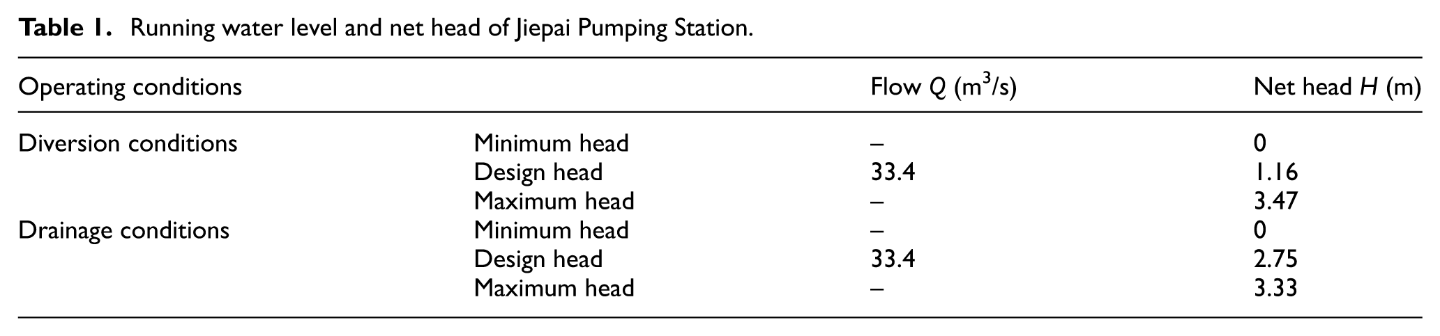
Jiepai Pumping Station is mainly for diversion, occasionally for drainage. The impeller diameter of each pump is 3.45 m and the rotating speed is 100 r/min. With the hydraulic loss of 0.2 m at gate slots and trash rack, the design head of diversion is 1.36 m and the highest head is 3.67 m, while the design head of drainage is 2.95 m and the highest head is 3.53 m.

Numerical simulation of pump device

Calculation model

A tank-style axial-flow pump device includes the following parts: inlet passage, impeller, guide vane, and outlet passage. The axial-flow pump used in this article is the GL-2008-03 hydraulic model developed independently by our project team. The design flow of this model pump Q = 320 L/s; the design head H = 2.5 m; the number of impeller blades is three. Diffusion guide vane is adopted in Jiepai Pumping Station, which matches the design flow of the axial-flow pump and its number is five. The diffusion angles of the guide vane hub and rim are both 12°. The blade angle for the computational configuration is −3°.

The numerical simulation is based on the prototype pump device:^14,15 the width of the inlet and outlet passages of the prototype pump device is B = 9.5 m (2.753D), height H = 4.4 m (1.275D), and length L = 37.5 m (10.87D). The inlet and outlet passages are modeled by UG, and the impeller and guide vanes are modeled by TurboGrid. Three-dimensional calculation model of axial-flow pump is shown in Figure 1.

Figure 1.

Numerical calculation model for pump device.

Grid division

ICEM is adopted to do the grid division of the inlet and outlet passages, and the quality of the grid is above 0.3, meeting the requirements of calculation. The impeller and diffuser vanes are divided into structural grids directly in TurboGrid, and the quality is good, meeting orthogonal requirements. The grids of the impeller and diffuser vanes are shown in Figure 2.

Figure 2.

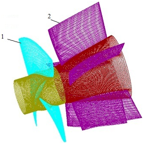
Impeller and guide vane grid chart.

Figure 3 shows the results of mesh independence examination for the axial-flow pump device. Six sets of computational mesh with mesh elements ranging from 1.0 × 10⁶ to 3.6 × 10⁶ are taken to test the mesh independence. The calculation results of pump head and efficiency demonstrate small difference when the mesh elements exceed 2.35 × 10⁶ (see Figure 3). To balance the computational accuracy and computational load, the set of computational mesh with 2,355,827 elements is chosen in the following calculations.

Figure 3.

Mesh independence check.

Boundary conditions

Three-dimensional unsteady Reynolds-averaged Navier–Stokes equations are applied to solve the turbulent flow in axial-flow pump device using a commercial software CFX. The renormalization group (RNG) k–ε model which is widely used in rotating fluid machinery is adopted in the numerical simulation. The flow inside the Jiepai pump device has a high strain rate and a large bending flow line. In such fluid machinery, RNG k–ε model has better analytical capabilities than other turbulence model. This model uses a statistical technique known as renormalization grouping, which corrects the turbulent viscosity by taking into account the rotation and swirl conditions, and adds to the ε equation an equation that reflects the time strain rate.^16–19

The scalable wall function is applied to calculate the turbulent flow near the solid walls. No-slip boundary conditions are imposed at the solid walls, such as the inlet and outlet passage walls, the blade pressure and suction surfaces, the hub and shroud, and the guide vane blade walls. The pressure at pump inlet and the mass flow at pump outlet are specified corresponding to the experimental measurement. The interfaces between the stable domain and rotational domain are set using the stage and the transient rotor–stator methods for steady and unsteady calculations, respectively. The relative position between the stable inlet passage and guide vane and the rotational impeller remain the same in the stage method, while it changes according to the angular velocity of the impeller in the transient rotor–stator method. The results of the steady calculation are taken as the initial flow field in the unsteady flow calculation.

For a tank-style pump device, the entrance of computational domain is the entrance of the inlet passage; the entrance boundary condition is set as the total pressure condition, that is, 1 standard atmospheric pressure. The exit of computational domain is the exit of the outlet passage; the exit boundary condition is set as mass flow. According to the literature,²⁰ the effects of time step on the unsteady simulation are minimal differences. Therefore, by considering the balance between the spectrum accuracy and the computation cost, we denote the final time step as 0.01 s.

Calculation formula

Hydraulic loss

The concept of hydraulic loss Δh is introduced according to the Bernoulli energy equation. The flow velocity field and the pressure field calculated by the computational fluid dynamics (CFD) numerical calculation are used to predict the hydraulic loss of the flow components, and the formula is as follows

Δ h = E_{1} - E_{2} = (\frac{P_{1}}{ρ g} - \frac{P_{2}}{ρ g} + Z_{1} - Z_{2}) + (\frac{u_{1}^{2}}{2 g} - \frac{u_{2}^{2}}{2 g})

(1)

where E₁ is the total energy at the entrance of the passage and E₂ is the total energy at the exit; P₁ is the static pressure at the entrance of the passage and P₂ is the static pressure at the exit; Z₁ is the height of the entrance of the passage and Z₂ is the height of the exit; u₁ is the flow velocity at the entrance of the passage and u₂ is the flow velocity at the exit; ρ is the water density; and g is the gravitational acceleration (m/s²).

Uniformity of axial velocity distribution at outlet section

The inlet passage should be designed to provide a uniform flow distribution and pressure distribution for the impeller. The uniformity (V_u) of the axial velocity distribution at the entrance reflects the design quality of the inlet passage. The closer the V_u is to 100%, the more uniform the axial-flow velocity distribution at the exit of the inlet passage. The calculation formula is as follows

V_{u} = {1 - \frac{1}{{\bar{v}}_{a}} \sqrt{\frac{[\sum_{i = 1}^{n} {(v_{a i} - {\bar{v}}_{a})}^{2}]}{n}}} \times 100 %

(2)

where V_u is the uniformity of axial-flow velocity distribution at the exit section of the inlet passage (%), v_a is the arithmetic mean value of the axial-flow velocity at the exit section of the inlet passage, v_ai is the axial velocity of each calculating unit of the exit section of the inlet passage (m/s), and n is the number of units on the exit section.

Performance prediction of pump

The head of pump device is calculated by Bernoulli energy equation. And the hydraulic performance of the pump device is predicted from the calculated velocity and pressure fields and the torque acting on the impeller. The pump head is expressed as follows

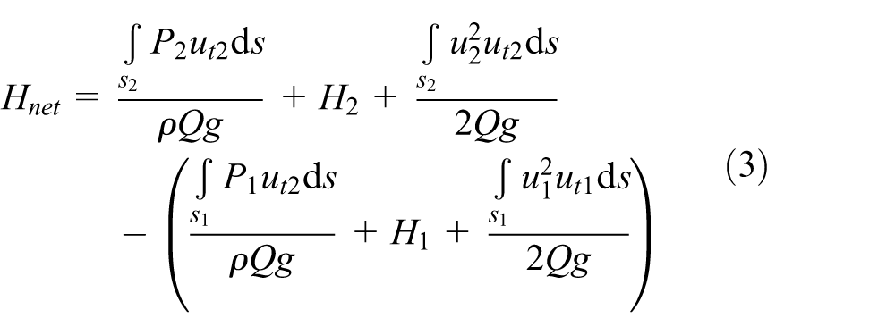
H_{n e t} = \frac{\int_{s_{2}} P_{2} u_{t 2} d s}{ρ Q g} + H_{2} + \frac{\int_{s_{2}} u_{2}^{2} u_{t 2} d s}{2 Q g} - (\frac{\int_{s_{1}} P_{1} u_{t 2} d s}{ρ Q g} + H_{1} + \frac{\int_{s_{1}} u_{1}^{2} u_{t 1} d s}{2 Q g})

(3)

where H₁ is the head of the inlet section and H₂ is the head of the outlet section (m); s₁ is the area of the inlet section and s₂ is the area of the outlet section (m²); u₁ is the flow velocity at each point on the section of the inlet passage and u₂ is the flow velocity at each point on the section of the outlet passage (m/s); u_t₁ is the normal component of velocity at each point on the section of the inlet passage and u_t₂ is the normal component of velocity at each point on the section of the outlet passage (m/s); P₁ is the static pressure at each point on the section of the inlet passage and P₂ is the static pressure at each point on the section of the outlet passage (Pa).

The efficiency of the pump device is as follows

η = \frac{ρ gQ H_{net}}{T_{p} ω}

(4)

where T_p is the torque (N m) and ω is the angular velocity of the impeller (rad/s).

Optimization of inlet and outlet passages

Orthogonal table

Orthogonal method is an important branch of statistics and widely used in industrial production and experiment. The most important step of the orthogonal method is to design the orthogonal table according to the specific problem. The orthogonal table includes two parts: (1) design factors and (2) factor levels. On the basis of five factors, a orthogonal table designation L16(45) is established, in which the individuals are 16 with five factors and four levels for each factor.

The test individuals in the orthogonal table are symmetrically and uniformly distributed to make sure the results can represent all the factor combinations. By referring the original inlet and outlet passages, the factor levels are determined as shown in Tables 2 and 4.

Table 2.

Design factors and levels of inflow passage.

Level	L₂₂ (m)	H₇₈ (m)	A₇₇ (°)	L₃₆ (m)	H₉₀ (m)
1	0.5	0.3	90	1	1.2
2	0.7	0.4	95	1.5	1.4
3	0.9	0.5	100	2	1.6
4	1.1	0.6	105	1.8	1.8

Optimization of inlet passage

The optimization of the inlet passage is based on the design conditions of forward diversion. Optimization design of local dimension mainly aims at the inlet flare tube and water guide cone. With parametric modeling, it is easy to implement model changes by modifying only a few parameters. The numerical simulation of the impeller and guide vane is done along with that of the inlet passage to ensure the reliability of the calculation results. DOE orthogonal experimental design is adopted to optimize the local dimension of the inlet passage. The control size is shown in Figure 4.

Figure 4.

Control size of inflow passage.

The five major dimensions in Figure 4 are used as design variables for DOE orthogonal test. These five design variables control the shape of the inlet flare tube and water guide cone of the inlet passage. Therefore, the parametric modeling is based on modifying the values of the five variables. The DOE analysis is aimed at the hydraulic loss (h) and the uniformity (V_u) of the axial velocity distribution of the inlet passage. The wall of the inlet passage is set as a rough wall, and the roughness is set to 2.5 mm. The factor levels are shown in Table 2. According to the above table, the orthogonal test is designed, and the calculation results are shown in Table 3.

Table 3.

Orthogonal design arrangement and result.

No.	L₂₂ (m)	H₇₈ (m)	A₇₇ (°)	L₃₆ (m)	H₉₀ (m)	h (cm)	V_u (%)
1	0.5	0.4	100	1.5	1.6	6.54	93.9
2	0.9	0.6	90	1.5	1.4	5.55	88.5
3	0.7	0.6	100	2	1.8	5.63	93.7
4	1.1	0.4	90	2	1.2	5.08	89.9
5	0.5	0.5	90	1.8	1.8	8.56	84.7
6	0.9	0.3	100	1.8	1.2	3.92	93.7
7	0.7	0.3	90	1	1.6	5.34	89.2
8	1.1	0.5	100	1	1.4	4.19	94.0
9	0.5	0.3	105	2	1.4	4.19	94.2
10	0.9	0.5	95	2	1.6	5.03	92.3
11	0.7	0.5	105	1.5	1.2	3.91	94.15
12	1.1	0.3	95	1.5	1.8	4.78	92.72
13	0.5	0.6	95	1	1.2	4.96	91.90
14	0.9	0.4	105	1	1.8	4.25	94.25
15	0.7	0.4	95	1.8	1.4	4.66	92.57
16	1.1	0.6	105	1.8	1.6	4.25	94.09
k ₁	6.06	4.56	6.13	4.68	4.46
k ₂	4.88	5.13	4.86	5.19	4.65
k ₃	4.68	5.42	5.06	4.98	5.29
k ₄	4.57	5.10	4.15	5.35	5.80
s ₀	1.37	0.86	1.98	0.66	1.34
Influence order: A₇₇ > L₂₂ > H₉₀ > H₇₈ > L₃₆
Excellent level 1.1		0.3	105	1	1.2	3.65	93.07

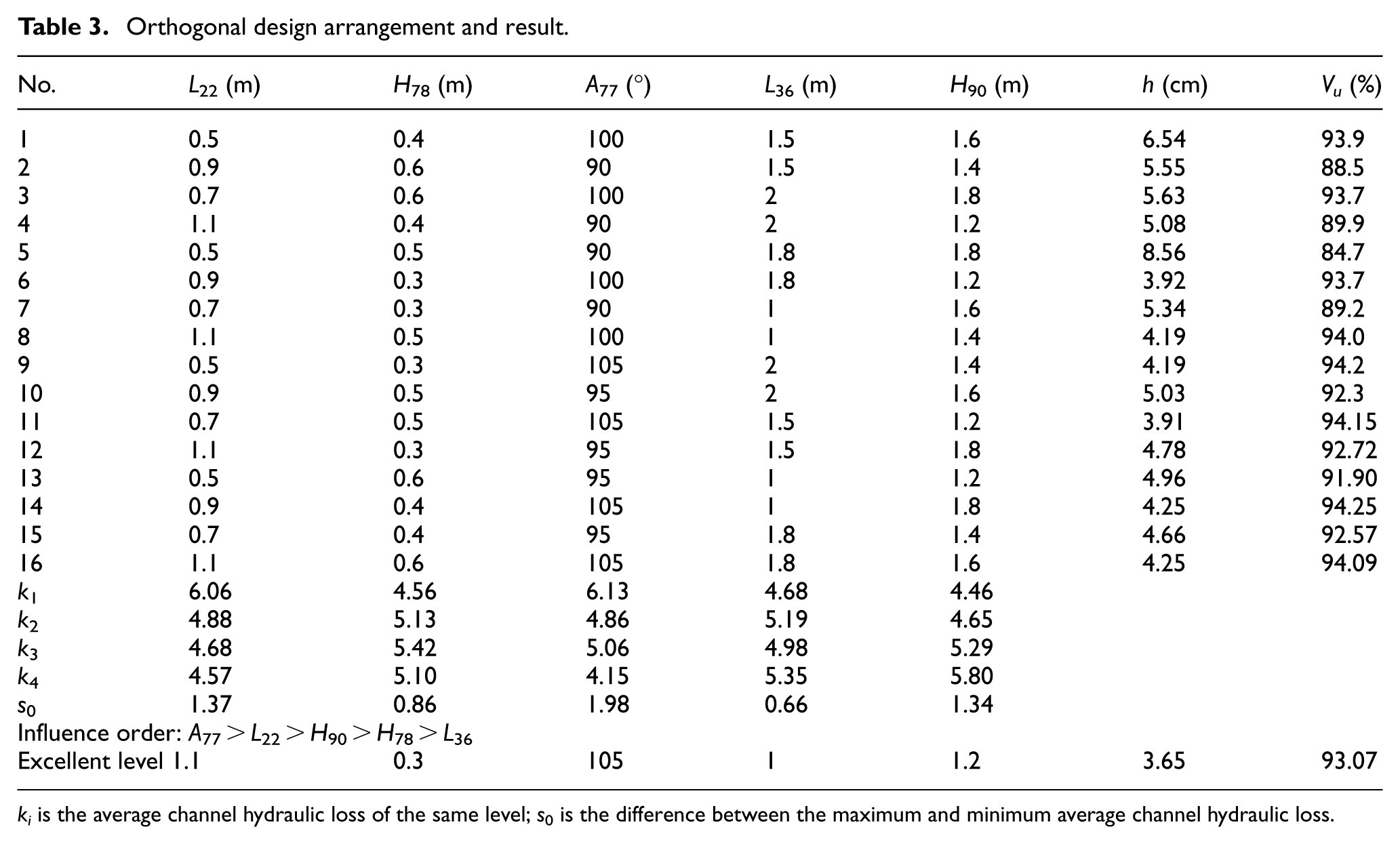
k_i is the average channel hydraulic loss of the same level; s₀ is the difference between the maximum and minimum average channel hydraulic loss.

According to the orthogonal design table above, the maximum hydraulic loss is 8.56 cm, while the minimum hydraulic loss is 3.91 cm, which is obviously a result of optimization. A₇₇ has the greatest impact on hydraulic loss, and L₃₆ has the least impact. The uniformity of velocity distribution upon the outlet section of the inlet passage is basically consistent with the trend of hydraulic loss. The maximum velocity distribution is 94%. According to the orthogonal design, the optimal combination should be 1.1, 0.3, 105°, 1, and 1.2 m. The initial scheme is no. 13, in which the hydraulic loss is 4.96 cm, and the outlet velocity uniformity is 91.9%. While in the optimal combination, the hydraulic loss is 3.65 cm and the outlet velocity uniformity is 93.0734%. Compared with the initial scheme, the optimal one reduces the hydraulic loss by 1.3 cm and improves the outlet velocity uniformity by 1.1%. The image extractions of exit section velocity of schemes 1, 5, and 13 and the optimal scheme are compared, as shown in Figure 5.

Figure 5.

The inlet and outlet section velocity diagram: (a) test no. 1, (b) test no. 5, (c) test no. 13, and (d) optimized result.

Seen from the axial velocity contours in Figure 5, the boundary velocities of all the four schemes are small due to the influence of the boundary layer of the wall of water guide cone and flare tube. Axial velocity has different distributions due to the influence of the structure of water guide cone and flare tube. No. 1 has a larger asymmetry in its axial velocity distribution and slightly more hydraulic loss than others. No. 5 has a larger low-velocity region of outlet flow, unreasonable speed distribution, and only 84.7% of the velocity uniformity; as a result, its hydraulic loss is much more than others. No. 13 has two low-speed regions, unsatisfactory design of the inlet flare tube, and water guide cone. Compared with them, the optimal scheme has more ideal velocity uniformity and velocity gradient, and its hydraulic loss is least.

Optimization of outlet passage

The outlet passage is parametrically modeled by UG, and just like inlet passage, the numerical simulation of outlet passage is also carried out with that of pump. In the process of optimization of the outlet passage, five factors were selected to design the orthogonal experiment. The parameterized model is shown in Figure 6.

Figure 6.

Parametric model of the outflow passage.

These five design parameters control the water guide cone and outlet flare tube of the outlet passage. Therefore, the parametric modeling is based on modifying the values of the five variables. The orthogonal design of these five factors is shown in Table 4.

Table 4.

Design factors and levels of outflow passage.

Level	P₄₉ (m)	P₅₄ (m)	P₄₇ (m)	P₅₃ (m)	P₄₆ (°)
1	3	1	1.6	1.1	80
2	3.4	1.1	2.0	1.3	78
3	3.8	1.2	2.4	1.5	76
4	4.2	1.3	2.8	1.7	74

The analysis of DOE orthogonal design aims at the hydraulic loss of the outlet passage. The wall of the outlet passage is set as rough wall, and the roughness is set to 2.5 mm. The orthogonal test analysis and the calculation results are shown in Table 5, based on the factor levels in Table 4.

Table 5.

Orthogonal design arrangement and results.

No.	P₄₉ (m)	P₅₄ (m)	P₄₇ (m)	P₅₃ (m)	P₄₆ (°)	Δh (cm)
1	3	1.1	2.4	1.3	76	42.83
2	3.8	1.3	1.6	1.3	78	41.22
3	3.4	1.3	2.4	1.5	74	43.47
4	4.2	1.1	1.6	1.5	80	38.68
5	3	1.2	1.6	1.7	74	45.52
6	3.8	1	2.4	1.7	80	32.70
7	3.4	1	1.6	1.1	76	37.38
8	4.2	1.2	2.4	1.1	78	39.37
9	3	1	2.8	1.5	78	39.97
10	3.8	1.2	2	1.5	76	33.87
11	3.4	1.2	2.8	1.3	80	36.44
12	4.2	1	2	1.3	74	36.41
13	3	1.3	2	1.1	80	41.51
14	3.8	1.1	2.8	1.1	74	46.07
15	3.4	1.1	2	1.7	78	37.94
16	4.2	1.3	2.8	1.7	76	38.66
k ₁	42.46	36.62	40.70	41.08	37.33
k ₂	38.81	41.38	37.43	39.23	39.63
k ₃	38.47	38.80	39.59	39.00	38.18
k ₄	38.28	41.22	40.29	38.70	42.87
s ₀	4.17	4.76	3.26	2.37	5.53
Influence order: P₄₆ > P₅₄ > P₄₉ > P₄₇ > P₅₃
Excellent level 4.2		1	2	1.7	80	32.53

P₄₆ has the greatest influence on the calculation results, and P₅₃ has the least influence. The hydraulic loss of the outlet passage calculated from the optimal level combination is 32.53 cm, while the maximum hydraulic loss is 46.07 cm; therefore, the hydraulic loss was reduced by 13.5 cm. The hydraulic loss of the initial outlet passage is 40.49 cm. Compared with the initial scheme, the optimized one reduces the hydraulic loss by 7.96 cm.

As noted in Figure 7, the static pressure value of the optimization scheme is larger than the others. It reveals the following facts: the dynamic pressure value in the outlet passage of the optimization scheme is smaller; the velocity is also smaller; optimized water guide cone and outlet flare tube are better able to recover outlet circulation of guide vane and more efficiently convert the kinetic energy into pressure energy; all the above leads to less hydraulic loss in the optimization scheme. The static pressure test no. 14 is smallest, indicating that it has the greatest hydraulic loss. Other findings are as follows: in each scheme, the pressure on the left wall along the direction of water flow is greater than that along the right wall, because water flow at the outlet of the flare tube, affected by the rotation of the impeller, will produce a drift, but the shock loss will be smaller with smaller velocity; five blades of the guide vane will result in five pressure concentration areas on the outlet flare tube and two pressure concentration areas on the right wall of the outlet passage along the flow direction; in test no. 1 and test no. 9, the two pressure concentration areas are very close to each other, and even overlapping, which will inevitably lead to the deterioration of the outflow condition of the corresponding region; in the optimized scheme, the two pressure concentration areas are far apart, which is one of the reasons for the less hydraulic loss. The pressure gradient of the optimized scheme is minimized, and the exit section of the outlet passage can obtain a higher pressure value by recovering velocity circulation, which are the reasons for the less hydraulic loss of the optimized scheme.

Figure 7.

Pressure distribution of outflow passage: (a) test no. 1, (b) test no. 9, (c) test no. 14, and (d) optimized result.

Analysis of calculation results of pump

The results of the DOE optimization were used to calculate the inlet and outlet passages of the tank-style pump device. Impeller diameter D is 3.45 m. The width of the inlet and outlet passages is 9.5 m, and the height is 4.4 m. The total length of the passage is 37.5 m. The blade angle of diversion condition is −3°, and the calculation conditions are 0.4Q₀, 0.5Q₀, 0.6Q₀, 0.7Q₀, 0.8Q₀, 0.9Q₀, 0.95Q₀, 1.0Q₀, 1.05Q₀, 1.1Q₀, and 1.15Q₀, and here, Q₀ is the design flow. The calculation model of the pump device is shown in Figure 8, and the results are summarized in Figures 9 –11.

Figure 8.

Calculation model of pump device.

Figure 9.

Prototype pump performance curves.

Figure 10.

Hydraulic loss curves of inflow and outflow passage.

Figure 11.

Blade axial thrust curve.

According to the pump performance curve, under the condition of diversion, the pump is running in the high-efficiency area, with the highest operating efficiency reaching 70.04%. Herein, the head is 1.736 m, and the maximum operating head is 4.0 m, which can meet the requirement of the maximum operating head of Jiepai Station, 3.67 m. When the running head is 1.36 m, the flow rate of the pump station is 34.31 m³/s and the efficiency is 66.82%. According to the hydraulic loss curve of the inlet and outlet passages, the hydraulic loss of the inlet passage increases with the increase in flow rate; the hydraulic loss of the outlet passage decreases first and then increases due to the existence of optimal circulation, wherein the hydraulic loss of the outlet passage is the least in the design condition. The axial force distribution curve is shown in Figure 11, wherein the axial thrust curve of the impeller is consistent with the trend of the head curve, and axial water thrust acting on the impeller is vertically down, and therefore, lift phenomenon will not occur when the pump operates normally.

Numerical calculation of pressure fluctuation

The relative movement between the rotating blade and the stationary blade, circular motion of the design conditions, cavitation, secondary flow, and other factors inside the axial-flow pump are all likely to produce pressure pulsation, which may intensify the structural vibration of the axial-flow pump device, lead to unstable operation of pump station. Therefore, it is necessary to find out the regularity of the water pressure pulsation of the bidirectional vertical pump device, so as to facilitate the safe and stable operation of the pump station.

When it comes to the unsteady calculation of the bidirectional vertical pump, the calculation is done on eight periods, and the results of the last five cycles are used to analyze pressure pulsation values. The pressure detection points are arranged at the key parts of the pump, including the water guide cone, the entrance of the impeller, the position between the impeller and the guide vane, and the exit of the guide vane. Four pressure pulsation detection points are arranged on each plane from the hub to the rim. By CFD, the pressure fluctuation time domain map and the frequency domain map at each pressure detection position are obtained, and thus, the water pressure pulsation characteristics of the key point are transparent. The arrangement of detection points is shown in Figure 12.

Figure 12.

Pressure detection point position.

Three flow conditions Q = 0.6Q₀, Q = Q₀, and Q = 1.15Q₀ are taken to analyze the pressure pulsation characteristics (Figures 13 –15).

Figure 13.

The pressure pulsation of the prototype pump device (Q = 20.04 m³/s): (a) the position of inlet flare tube, (b) the position of the entrance of impeller, (c) the position between impeller and guide vane, and (d) the position of the exit of guide vane.

Figure 14.

The pressure pulsation of the prototype pump device (Q = 33.4 m³/s): (a) the position of inlet flare tube, (b) the position of the entrance of impeller, (c) the position between impeller and guide vane, and (d) the position of the exit of guide vane.

Figure 15.

The pressure pulsation of the prototype pump device (Q = 38.41 m³/s): (a) the position of inlet flare tube, (b) the position of the entrance of impeller, (c) the position between impeller and guide vane, and (d) the position of the exit of guide vane.

The pressure fluctuation curves of the detection points at the inlet flare tube and the entrance of impeller are regular and smooth. The pressure pulsation curve of the four inspection points between the impeller and guide vane is slightly disordered due to the static and dynamic interference between the impeller and the guide vane. The pressure pulsation curve of the eight inspection points at the exit of guide vane is not smooth, and a large amplitude of the low-frequency pressure pulsation occurs, which indicates that there exists de-flow at these detection points. Meanwhile, the four detection points along the circumference have quite different pressure fluctuation and amplitude, which may be caused by the remaining velocity circulation of the guide vanes.

The main frequency of the three monitoring surfaces between the inlet flare tube, impeller inlet, and impeller guide vane is three times the impeller rotational frequency, which indicates that the pressure fluctuation of the flow in the axial-flow pump is determined by the frequency of the blade. The flow frequency of guide vane outlet, outlet flare tube, and outlet passage is 5 Hz with low-frequency pulsation, which is caused by flow separation.

Different monitoring points have different pressure fluctuation amplitude. The one at the impeller inlet is the largest, which is caused by a larger pressure difference between the front and rear sides of the blade. The amplitude of pressure fluctuation at other locations is smaller. Therefore, in the future hydraulic design process, great importance should be attached to inlet pressure pulsation of axial-flow pump.

The pressure pulsation amplitude of the inlet flare tube decreases with the increase in flow rate. The pressure pulsation amplitude of different flow conditions is smaller. The pressure pulsation amplitude of the impeller inlet is the largest that decreases with the increase in flow rate. The pressure pulsation amplitude under the small flow condition is about 1.8 times higher than that under the design flow condition and 2.1 times higher than that under the large flow conditions. That illustrates the pressure pulsation of the impeller inlet is larger due to its import pressure difference. The pressure pulsation amplitude between the impeller and the guide vane is smaller than that of the impeller inlet. With the increase in flow rate, the pressure fluctuation amplitude between the impeller and the guide vane decreases first and then increases. There is no obvious regularity between the pressure fluctuation amplitude and the flow rate of guide vane outlet.

According to the frequency spectrum, it can be seen that the pressure pulsation at the inlet flare tube, impeller inlet, and between the impeller and the guide vane is mainly affected by the blade rotation. The water flow is stable and periodic in these areas. Therefore, the main frequency of the pressure pulsation depends on the blade frequency. The similarity of the pressure fluctuation at the guide vane outlet is bad, because low-frequency pulsation will be produced in addition to the impact of blade frequency, which is due to the regional water flow instability.

Experimental verification

According to the final optimization scheme obtained by the numerical simulation of tank-style pump device, the flow passage, impeller, and guide vane are machined, and model test study is carried out on the high-precision vertical closed cycle hydraulic mechanical test bench in Yangzhou University. Model pump nominal impeller diameter D is 300 mm, the actual impeller diameter D is 299.7 mm, and blade number of guide vane is 5, which is welded with steel material. To facilitate observation of internal water flow patterns, the observation window is opened in the impeller chamber and the passage wall. Pump segment model installation checking is as follows: the axial runout is set to 0.10 mm for the positioning surface of guide vane and impeller chamber, the radial runout is set to 0.08 mm for the outer surface of the impeller hub, and the unilateral clearance of the blade tip is controlled within 0.20 mm. The model pump speed is 1150 r/min. The test platform is shown in Figure 16. The model pump device test is shown in Figure 17.

Figure 16.

High-precision hydraulic mechanical test bench.

Figure 17.

Model pump device test: (a) impeller, (b) guide vane, and (c) pump device.

The total length of the hydraulic closed circulation system is 60 m, pipe diameter is 0.5 m, and the comprehensive error of efficiency test system is about 0.39%. Referring to relevant procedures, performance test points of each blade angle are not less than 18; the required net positive suction head (NPSH) is determined by 1% reduction in efficiency.

The energy performance and cavitation performance of the six blade angle, namely, −4°, −3°, −2°, 0°, 2°, and 4°, are tested. The experimental results about the model pump device are shown in Figure 18.

Figure 18.

Comprehensive characteristic curves of pump device.

The maximum efficiency of the pump device is 71.9% while it occurs in the experiments (−3°). The blade angle of the numerical model pump is also −3°, which is the design angle under the forward diversion conditions. It can meet the design requirement of the flow and head. And the optimization design of the inflow and outflow passages is under the blade angle, so the efficiency of the pump device under the blade angle is the highest. The highest efficiency values of other blade angles are slightly lower. The necessary NPSH near the area of the design condition is relatively small, indicating that the cavitation performance is the best. The farther the necessary NPSH is away from the design condition, the worse the cavitation performance will be.

The conversion formulas of the numerical simulation results of the prototype pump and the model pump characteristics are as follows

\frac{Q_{p}}{Q_{m}} = \frac{n_{p} {D_{p}}^{3}}{n_{m} {D_{m}}^{3}}

(5)

\frac{H_{p}}{H_{m}} = \frac{{n_{p}}^{2} {D_{p}}^{2}}{{n_{m}}^{2} {D_{m}}^{2}}

(6)

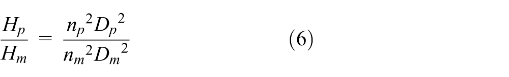
where Q_p is the prototype pump flow and Q_m is the model pump flow; H_p is the prototype pump head and H_m is the model pump head; n_p is the prototype pump speed and n_m is the model pump speed; D_p is the impeller diameter of prototype pump and D_m is the impeller diameter of model pump.

The results of the test data with blade angle of −3 ° are taken out and compared with the numerical simulation results, as shown in Figure 19.

Figure 19.

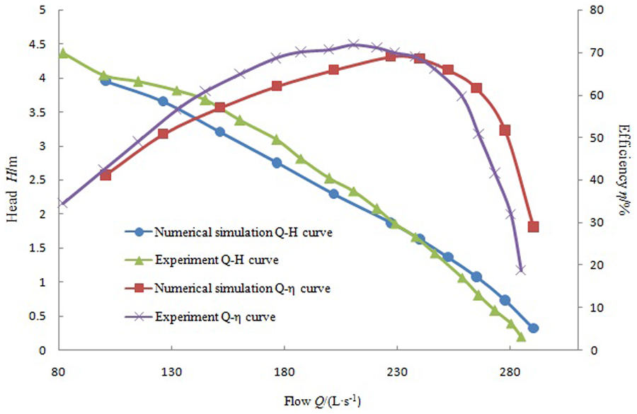
Comparison between test data and numerical simulation results.

It can be seen from the comparison chart of test data and numerical simulation results that the two curves coincide well in the vicinity of the design point. The highest operating efficiency of the test results reaches 71.5%; the corresponding head is 2.3 m, which is a little higher than the simulated one. According to engineering experience,^5,8 at present, the highest efficiency of the same type of pump device is about 70%, and the corresponding head is 4–5 m. After optimization, the efficiency of the test is more than 71% when the head is 2.3 m. The test operation efficiency is about 64% when the design head is 1.36 m, which is in good agreement with the numerical simulation results. The calculation result is low in small flow area and high in large flow area, but the trend of the whole performance curve is relatively good, which is able to meet the requirements of engineering application. It also shows that the orthogonal design used in this article to optimize flow channel is effective and feasible, and thus, it can provide reference for similar pump station project.

Conclusion

The orthogonal design, based on parametric modeling and used to optimize the inlet and outlet passages of tank-style pump device, can get better optimization results and shorten the optimal design cycle. After orthogonal design optimization, the hydraulic loss of the inlet passage of the tank-style pump device is reduced by 1.3 cm, and the hydraulic loss of the outlet passage is reduced by 7.96 cm; the test operation efficiency is about 64% when the design head is 1.36 m; the highest operating efficiency of the test results reaches 71.5%. The optimization effect of the pumping station is very obvious in the ultra-low lift vertical pump device. The highest pressure fluctuation appears at the entrance of the impeller, which is caused by a larger pressure difference between the front and rear sides of the blade; the main pressure fluctuation frequency of is 5 Hz, depending on the frequency of the blade. The pressure pulsation amplitude of the inlet flare tube and the entrance of the impeller decrease with the increase in flow rate. With the increase in flow rate, the pressure fluctuation amplitude between the impeller and the guide vane decreases first and then increases. There is no obvious regularity between the pressure fluctuation amplitude and the flow rate of guide vane outlet.

Footnotes

Academic Editor: M Affan Badar

Declaration of conflicting interests

The author(s) declared no potential conflicts of interest with respect to the research, authorship, and/or publication of this article.

Funding

The author(s) disclosed receipt of the following financial support for the research, authorship, and/or publication of this article: The research was supported by the National Natural Science Foundation of China (grant nos 51376155, 51609210), the National Science & Technology Support Project of China (grant no. 2012BAD08B03-2), a project funded by the Priority Academic Program Development of Jiangsu Higher Education Institutions (PAPD), and Jiangsu Province scientific research and innovation project (grant no. KYLX15_1365), and the open research subject of Key Laboratory of Fluid and Power Machinery, Ministry of Education (szjj2016-078).

References

Zhu

Zeng

. Experimental study on two-way flow passages in pumping system. J Mech Sci Technol 2008; 22: 1966–1970.

Liu

Jin

Zhou

. Numerical simulation and experimental study of a two-floor structure pumping system. In: Proceedings of the ASME power conference, Chicago, IL, 13–15 July 2010, pp.777–784. New York: ASME.

Chen

Zhou

. Study on hydraulic characteristics of tank-style outlet passage in low water head pumping stations. Trans Chin Soc Agric Mach 2007; 38: 70–72.

Cheng

Liu

. Advances in research on flow characteristics and hydraulic performances of low lift head pumping station. Adv Sci Tech Water Res 2008; 28: 85–88.

Yang

Liu

Tang

. Analysis on pressure fluctuation of interior flow in reversible pumping system for irrigation and drainage. J Drain Irrig Mach Eng 2011; 29: 316–321.

Liu

. Hydraulic performance assess target research of low-head pump equipment in south-north water transfer project. J Drain Irrig Mach Eng 2014; 21: 2–5.

Yan

. Research on efficient pump device with new type volute passage of large pumping station. J Hydroelectr Eng 2009; 28: 200–205.

Huang

Zhang

. Hydrodynamic optimization of large pump installation with two-way channel and experiment. J Drain Irrig Mach Eng 2016; 34: 602–607.

Chen

Wang

. Design of reversible passage in large axial pumping stations and experimental research on the characteristics of pump sets. J Jiangsu Univ Sci Tech: Nat Sci 2001; 22: 44–49.

10.

Yang

Liu

Tang

. Analysis of hydraulic performance for vertical axial-flow pumping system with cube-type inlet passage. Trans Chin Soc Agric Eng 2014; 30: 62–69.

11.

Tan

Zhu

Cao

. Numerical simulation of unsteady cavitation flow in a centrifugal pump at off-design conditions. Proc IMechE, Part C: J Mechanical Engineering Science 2014; 228: 1994–2006.

12.

Tan

Zhu

Wang

. Numerical study on characteristics of unsteady flow in a centrifugal pump volute at partial load condition. Eng Computation 2015; 32: 1549–1566.

13.

Tan

Cao

. Numerical investigation of clocking effect on a centrifugal pump with inlet guide vanes. Eng Computation 2016; 33: 465–481.

14.

Tang

Wang

Liu

. Design and numerical analysis on an axial-flow model pump with high specific speed. Chinese J Mech Eng 2005; 41: 119–123.

15.

Shi

Tang

Xie

. Design of axial flow pump modification and its effect based on CFD calculation. Trans Chin Soc Agric Eng 2015; 31: 97–102.

16.

Bryne

Taguchi

. The Taguchi approach to parameter design. Qual Prog 1987; 20: 19–26.

17.

Rao

Kumar

Prakasham

. The Taguchi methodology as a statistical tool for biotechnological applications: a critical appraisal. Biotechnol J 2008; 3: 510–523.

18.

Yakhot

Orzag

. Renormalization group analysis of turbulence: basic theory. J Sci Comput 1986; 1: 3–11.

19.

Wang

. Research progress of computational model for rotating turbulent flow in fluid machinery. Trans Chin Soc Agric Mach 2016; 47: 1–14.

20.

Wang

Tan

Zhu

. Numerical investigation of influence of inlet guide vanes on unsteady flow in a centrifugal pump. Proc IMechE, Part C: J Mechanical Engineering Science 2015; 229: 3405–3416.

Numerical and experimental investigation of tank-type axial-flow pump device

Abstract

Keywords

Introduction

General situation of pumping station

Numerical simulation of pump device

Calculation model

Grid division

Boundary conditions

Calculation formula

Hydraulic loss

Uniformity of axial velocity distribution at outlet section

Performance prediction of pump

Optimization of inlet and outlet passages

Orthogonal table

Optimization of inlet passage

Optimization of outlet passage

Analysis of calculation results of pump

Numerical calculation of pressure fluctuation

Experimental verification

Conclusion

Footnotes

Declaration of conflicting interests

Funding

References