Analysis method of dynamic response in the whole process of the vehicle bump test of simply supported bridge

Abstract

For medium- and small-span bridges, the vehicle bump test is one of the most commonly used excitation methods, dynamic response of which can provide theoretical support for the dynamic load test. This article presents a dynamic response analysis method for the whole process of the vehicle bump test. First, the process of vehicle bump is divided into three stages based on transformation of the vehicle–bridge contact condition, including the static state before vehicle bump, the process of vehicle bump, and the free-decay vibration after vehicle bump. Second, the vibration equations of each stage are established, respectively, on the basis of the characteristics of vehicle–bridge coupling vibration. Then, the starting time and initial conditions of each stage are determined and the dynamic response is estimated by the fourth-order Runge–Kutta method. Finally, a field experiment is carried out; the error of the maximum strain value between the proposed method and the test method is less than 15%, which perfectly verifies the reliability of the method. The dynamic response of a T-shaped simply supported bridge of the whole vehicle bump process is solved by numerical simulation which indicates that the proposed method can provide theoretical basis for the choice of vehicle bump height.

Introduction

The natural frequency, modal shape, damping ratio, impact coefficient, and so on, are very important for bridge design, state evaluation, and damage identification. Dynamic load test is one of the most effective methods to determine these dynamic parameters of bridges. In dynamic load test, different excitation methods are used to excite different bridge structures in order to make the bridge produce obvious vibration effect. There are three kinds of excitation methods for bridge structures: free vibration method, forced vibration method, and ambient excitation method.^1–8 Free vibration method includes impact excitation, ¹ step relaxation test, ² vehicle bump test, ³ by imposing the initial displacements, ⁴ and so on, while forced vibration method contains electrohydraulic shakers and ⁵ moving vehicle test ⁶ with ambient excitation comprising seismic ground motion, wind, and waves. ⁷ Farrar et al. ⁸ carried out a comprehensive summary and analysis with excitation methods of bridge structure. Mazurek ⁹ outlined the application of ambient excitation method in bridge detection, and the experimental study of aluminum slab beam bridge was carried out based on this method.

For small- and medium-span bridge structures, moving vehicle test and vehicle bump test are two of the most commonly used excitation methods. Moving vehicle test is to pass through the bridge with vehicle to produce forced vibration, and sometimes obstacles are placed on the deck in order to increase the input to the bridge. IR Racanel ¹⁰ artificially produced an obstacle on the bridge so that the superstructure of the bridge can produce an impact force under dynamic loads. H Alaylioglu and A Alaylioglu ¹¹ placed wooden planks across the central line of the bridge deck, and vibration tests of different vehicles at different speeds were carried out to obtain dynamic response characteristic. The vehicle bump test is to place the front or rear wheels of the vehicle on a certain height obstacle and then make it fall suddenly, which is equivalent to imposing an impulsive force on the bridge to make the bridge produce free attenuation vibration, and the position of the vehicle remains unchanged throughout the whole test. Vehicle bump test is favored by engineers and technicians in China, probably because this excitation method makes the vibration of the bridge structure more obvious and the collected dynamic response of bridge is a free attenuation response. ¹² In the dynamic test of Huang et al., ¹³ the impact force of the beam is caused by the fall of the rear wheel of a 14-ton truck from the concrete block. For different bridges, how to choose a suitable height of obstacle (also called height of vehicle bump in this article) is a difficult technical problem for engineers and technicians. If the height of the obstacle is too high, it may cause additional damage to the bridge structure, especially to the damaged bridge. If the height is too small, the vibration of the bridge structure is not obvious, which leads to the low signal-to-noise ratio of the collected dynamic response. “Industry Standards of Transport Ministry” (trial version) in 1982 ¹⁴ suggested that the obstacle height should be 5–15 cm when a single vehicle is excited by a heavy vehicle. “Industry Standards of Transport Ministry” (Final recommendations) in 2013 ¹⁵ regulated that the obstacle height should be 5–10 cm. These two standards are both aimed at long-span concrete bridges, while there is no regulation on the height of vehicle jump for medium- and small-span bridges at present. The dynamic response analysis of the whole process of the vehicle bump test can not only provide a theoretical basis for the vibration excitation method but also help engineers and technicians to choose the appropriate height of vehicle bump.

In essence, the whole process dynamic response analysis of the vehicle bump test is also a vehicle–bridge-coupled vibration problem, which can be traced back to the 1920s. It goes through three stages: the moving force,^16,17 the moving mass,^18,19 and the moving spring–mass system. ²⁰ The interest in the study of vehicle–bridge coupling vibration has been increasing, and more and more attention has been paid to the study of complex vehicle–bridge coupling vibration in the past few decades. The complexity of the vehicle–bridge coupling vibration problem lies in the vehicle model, the bridge model, the contact condition of the wheel, and the bridge structure, and so on. In terms of vehicle models, Lou and Zeng ²¹ use multi-rigid-body system to build railway freight vehicle model. Li et al. ²² adopted a three-dimensional system composed of mass–spring–damper of 11 degrees to represent a vehicle. The study of vehicle–bridge coupling vibration of many kinds of complex bridge structures has been studied. Wang et al. ²³ analyzed the dynamic characteristics of multi-span continuous bridge under the dynamic interaction of traffic and vehicle based on the complex bridge system and complex vehicle model and An et al. ²⁴ also took long-span continuous girder bridge as research object; Zhong et al. ²⁵ selected the prestressed bridge as research object; Nguyen ²⁶ researched the cracked beam-like bridge; Wang et al. ²⁷ studied on vehicle coupling vibration of four different types of cable-stayed bridges; and Song et al. ²⁸ discussed the cable-stayed bridge under moving vehicles with different speed and mass. The research on the contact conditions is focused on the roughness of the tire and the road surface, and so on. Zhang et al. ²⁹ put forward a nonlinear multi-spring tire model and Meng et al. ³⁰ analyzed the nonlinear properties of the bridge under a passing vehicle; Zhang et al. ³¹ proposed an approach in order to simulate the road roughness.

In fact, the above references discussed the solution of the dynamic response of the bridge structure when the vehicle moves on the bridge structure. Although the vehicle moves along the length of the bridge structure, all the wheels are always in contact with the bridge deck. But in the process of the vehicle bump test, the front wheels of the vehicle always contact with the bridge deck, while the rear wheels go through a process of contact, separation, and re-contact with the bridge deck, which will undoubtedly increase the complexity of solving the dynamic response. It can be considered that vehicle bump test is a special vehicle–bridge-coupled vibration problem, but the methods proposed in the above references cannot be directly used to solve this problem. The author of this article has proposed a theoretical method to determine the height of vehicle bump on the basis of the dynamic response of bridge structure.^32,33 The falling process of rear wheel is approximated as a vehicle–bridge momentum transformation process when solving the dynamic response in this method, and the variation of the motion parameters (displacement, velocity, acceleration) of each degree of freedom in the bridge structure and vehicle model is ignored in this process, which will result in errors in the solution of dynamic response, and the method cannot solve the whole process dynamic response of the bridge structure in vehicle bump test.

In view of the above problems, this article has carried out the further research. First, the vehicle bump test is divided reasonably. Second, the vehicle–bridge coupling vibration equation is established, then the starting time and initial conditions of each stage are determined. In the light of the calculation, the dynamic response of the whole process of the vehicle bump test is estimated by Runge–Kutta method. Finally, field tests and numerical example are carried out to verify the effectiveness of the proposed method. The greatest innovation of this article is to put forward an accurate method to estimate the dynamic response in the whole process of the vehicle bump test, which can provide theoretical basis for the determination of vehicle bump height and function as a technical support for the vehicle bump test.

Theoretical background

Simplified vehicle and bridge models

Small- and medium-span bridges are the most commonly used simply supported beams which can be split into integral bridge and multi-beam bridge in the light of the composition of main girder. For the whole bridge, only one main beam determines the mechanical properties of the bridge. For multi-beam bridges, horizontal connections between beams are used to withstand loads. It is apparent from Figure 1 that the mechanical properties of multi-beam structures are determined by the combination of all beams.

Figure 1.

Cross-sectional sketch of multi-beam bridge.

In general, the multi-beam bridge is one of the most commonly used bridges in the small and medium simply supported beam bridges, dynamic response analysis of which should be carried out for each main beam.

Based on the recent research, the transverse distribution coefficient of load is a hinge that simplifies the overall mechanical properties of multi-beam bridges on the mechanical properties of single beam, and the commonly used methods to calculate the transverse distribution coefficient of bridge load are the eccentric compression method, level principle method, hinge-jointed plate girder method, and so on. ³⁴ As a result, the load of the multi-beam bridge is converted into a single beam for calculation, and the space model is simplified into a plane model using the transverse distribution coefficient in the vehicle bump test.

The vehicle model with 4 degrees of freedom and 6 degrees of freedom is suitable for single beam and space beam, respectively. The plane single beam structure is adopted in this article, so 4-degree-of-freedom half-car plane model is selected.

Decomposition of the process of vehicle bump test

The vehicle bump test is decomposed into different stages for the following analysis in this article. As can be seen in Figures 2–4, these three stages of the static state before vehicle bump (Stage I), the process of vehicle bump (Stage II), and the free-decay vibration after vehicle bump (Stage III) are demonstrated, respectively. The critical state given in Figure 5 is chosen as the reference system for force analysis and coordinates of all degrees of freedom for three stages; that is, the vehicle wheels are in contact with bridge, but the springs are not compressed and the bridge has no static displacement.

Figure 2.

The static state before vehicle bump (Stage I).

Figure 3.

The process of vehicle bump (Stage II).

Figure 4.

The free-decay vibration after vehicle bump (Stage III).

Figure 5.

The reference system of critical state.

As can be seen in Figures 2–4, $m_b$ , $m_{t1}$ , $m_{t2}$ stand for the masses of vehicle body, front, and rear wheels, respectively; $r_1$ , $r_2$ are the distances between front and rear axles and centroid of vehicle body, respectively; $k_a$ , $k_t$ are the stiffness coefficients of tires and suspensions; θ is rotation angle of the vehicle body; $y_b$ , $y_{t1}$ , $y_{t2}$ are the vertical displacement of vehicle body, front, and rear wheels, respectively; and $y_1$ , $y_2$ represent the deflections of the bridge at the position of the front and rear wheels, respectively. a stands for the axle spacing; h is the height of vehicle bump; c represents distance between coordinate origin and rear wheel; $c_a$ , $c_t$ are the damping coefficients of tires and suspensions.

Calculation models for dynamic response of three stages

Dynamic equation of Stage I

As is exhibited in Figure 2, the front wheel is on the bridge and the rear wheel is located at the height h of the obstacle, which is the static state before vehicle bump.

Let p₁ and p₂ be the vehicular loads of front and rear wheels, respectively, which can be evaluated as follows

$$p_1=\varphi [m_{t1}g+\frac{r_2}{r_1+r_2}·m_{b}g]$$

(1a)

$$p_2=\varphi [m_{t2}g+\frac{r_1}{r_1+r_2}·m_{b}g]$$

(1b)

where ϕ indicates the load transverse distribution coefficient of single beam in the whole bridge.

Let the static state in Figure 2 be the initial moment of vehicle bump test, that is, the moment t = 0. The static displacement of the bridge $y_{p1}(x)$ and $y_{p2}(x)$ at the position of x generated by $p_1$ and $p_2$ , respectively, is given by $y_{p2}(x)$

$$y_{p_1}(x,0)=\{\begin{array}{c}\frac{p_1(l-c+a)x}{6\mathrm{EIl}}[l^2-x^2-{(l-c+a)}^2],0⩽x⩽c-a\hfill \\ \multicolumn{1}{c}{\frac{p_1(l-c+a)}{6\mathrm{EIl}}\{\frac{l}{l-c+a}{[x-(c-a)]}^3+[l^2-{(l-c+a)}^2]x-x^3\},c-a⩽x⩽l}\end{array}$$

(2)

$$y_{p_2}(x,0)=\{\begin{array}{c}\frac{p_2(l-c)x}{6\mathrm{EIl}}[l^2-x^2-{(l-c)}^2],0⩽x⩽c\hfill \\ \multicolumn{1}{c}{\frac{p_2(l-c)}{6\mathrm{EIl}}\{\frac{l}{l-c}{(x-c)}^3+[l^2-{(l-c)}^2]x-x^3\},c⩽x⩽l}\end{array}$$

(3)

where EI indicates the flexural rigidity of the bridge; l stands for the length of bridge.

Then, the static displacement of the bridge in Stage I can be obtained by

$$y(x,0)=y_{p1}(x,0)+y_{p2}(x,0)$$

(4)

According to the reference system in section “Decomposition of the process of vehicle bump test,” the initial displacements of 4 degrees of freedom of vehicle system in Stage I can be gained in the following (i.e. the springs are compressed and the bridge has static displacement)

$$\{\begin{array}{c}{y}_{t1}=y_1(0)+\frac{(\frac{r_2}{r_1+r_2}{m}_{b}g+m_{t1}g)}{k_{a1}}\hfill \\ \multicolumn{1}{c}{y_{t2}=y_2(0)-h+\frac{(\frac{r_1}{r_1+r_2}{m}_{b}g+m_{t2}g)}{k_{a2}}}\\ \multicolumn{1}{c}{y_b=\frac{\{r_{1}y{t}_2+(a-r_1)y{t}_1+\frac{[t_1{r}_1^2+t_2(a{r}_1-r_1{r}_2)]m_{b}g}{k{t}_1{t}_2(r_1+r_2)}\}}{a}}\\ \multicolumn{1}{c}{\theta =\frac{[y{t}_2-y{t}_1+\frac{(t_1{r}_1-t_2{r}_2)m_{b}g}{k{t}_1{t}_2(r_1+r_2)}]}{a}}\end{array}$$

(5)

Vehicle–bridge coupling vibration equation of Stage II

The process of vehicle bump is presented in Figure 3, that is, the rear wheels abruptly fell off the obstacle with height h without horizontal velocity and the front wheels produce vibration with the contact point between front wheels and bridge structure.

The vehicular load of front wheel acting on the bridge of Stage II can be expanded as follows

$$p(t)=\phi [c_{a1}({\stackrel{·}{y}}_{t1}-{\stackrel{·}{y}}_1)+k_{a1}(y_{t1}-y_1)]$$

(6)

As can be observed in Figure 3, the bridge is considered as an Euler–Bernoulli beam. We can obtain

$$m\stackrel{··}{y}(x,t)+C\stackrel{·}{y}(x,t)+\mathrm{EI}\frac{{\partial }^{4}y(x,t)}{\partial x^4}=p(t)\delta (x-(c-a))$$

(7)

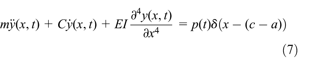
Equation (7) is the equation of motion for the bridge structure, where m, C, y(x, t) $\delta$ are the mass per unit length, the damping, the dynamic displacement function of the bridge, and Dirac delta function, respectively.

Let

$$y(x,t)=\sum _i^n{\varphi }_i(x)q_i(x)$$

(8)

where ${\varphi }_i(x)$ is the ith-order mode shape function of simply supported bridge, which is determined by the eigenvalue and eigenfunction analysis.

Combining equations (7) and (8), integrating with respect to x between 0 and l, the following results can be obtained

$$\begin{array}{c}\multicolumn{1}{c}{\underset{0}{\overset{l}{\int }}m{\varphi }_i^2(x){\stackrel{··}{q}}_t(t)\mathrm{dx}+\underset{0}{\overset{l}{\int }}2\beta m{\varphi }_i^2(x){\stackrel{·}{q}}_t(t)\mathrm{dx}+{\omega }_i^2}\\ \multicolumn{1}{c}{\underset{0}{\overset{l}{\int }}m{\varphi }_i^2(x)q_i(t)\mathrm{dx}=\underset{0}{\overset{l}{\int }}{\varphi }_i(x)p(t)\delta (x-(c-a))\mathrm{dx}}\end{array}$$

(9)

where ${\omega }_i$ is the ith natural frequency; $\beta =C/2m$ . Let $s_i={\int }_0^{l}m{\varphi }_i^2(x)\mathrm{dx}$ , and we can describe equation (9) as follows

$$s_i{\stackrel{··}{q}}_i(t)+2\beta s_i{\stackrel{·}{q}}_i(t)+{\omega }_i^2{s}_i{q}_i(t)={\varphi }_i(c-a)p(t)$$

(10)

Wheel masses $m_{t1}$ and $m_{t2}$ can be solved as follows

$$\begin{array}{c}\multicolumn{1}{c}{m_{t1}{\stackrel{··}{y}}_{t1}+c_{a1}({\stackrel{·}{y}}_{t1}-{\stackrel{·}{y}}_1)+k_{a1}(y_{t1}-y_1)+c_{t1}({\stackrel{·}{y}}_{t1}-{\stackrel{·}{y}}_b}\\ \multicolumn{1}{c}{+r_1\stackrel{·}{\theta })+k_{t1}(y_{t1}-y_b+r_1\theta )=m_{t1}g}\end{array}$$

(11a)

$$m_{t2}{\stackrel{··}{y}}_{t2}+c_{t2}({\stackrel{·}{y}}_{t2}-{\stackrel{·}{y}}_b-r_2\stackrel{·}{\theta })+k_{t2}(y_{t2}-y_b-r_2\theta )=m_{t2}g$$

(11b)

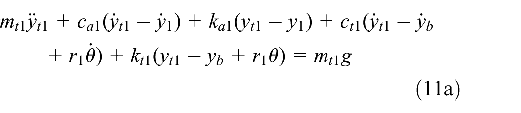
The linear force balance equations for vehicle body are listed as follows

$$\begin{array}{c}\multicolumn{1}{c}{m_b{\stackrel{··}{y}}_b+k_{t1}(y_b-y_{t1}-r_1\theta )+c_{t1}({\stackrel{·}{y}}_b-{\stackrel{·}{y}}_{t1}-r_1\stackrel{·}{\theta })}\\ \multicolumn{1}{c}{+k_{t2}(y_b-y_{t2}+r_2\theta )+c_{t2}({\stackrel{·}{y}}_b-{\stackrel{·}{y}}_{t2}+r_2\stackrel{·}{\theta })=m_{b}g}\end{array}$$

(12a)

$$\begin{array}{c}\multicolumn{1}{c}{I_b\stackrel{··}{\theta }-r_1[c_{t1}({\stackrel{·}{y}}_b-{\stackrel{·}{y}}_{t1}-r_1\stackrel{·}{\theta })+k_{t1}(y_b-y_{t1}-r_1\theta )]}\\ \multicolumn{1}{c}{+r_2[c_{t2}({\stackrel{·}{y}}_b-{\stackrel{·}{y}}_{t2}+r_2\stackrel{·}{\theta })+k_{t2}(y_b-y_{t2}+r_2\theta )]=0}\end{array}$$

(12b)

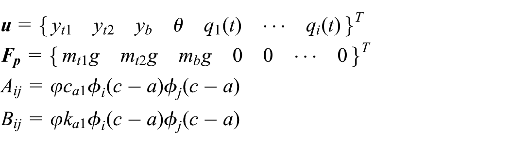
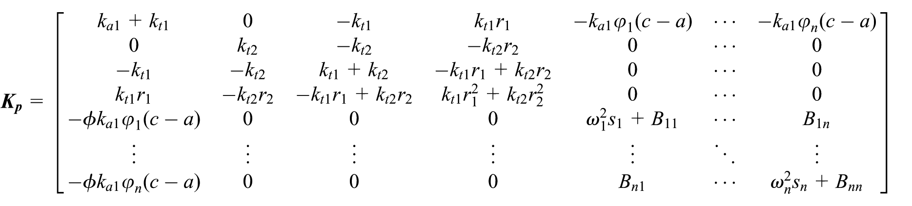
Combining equation (7) and equations (10)–(12), the vehicle–bridge coupling system generalized equation of motion in Stage II could be expressed in matrix form; it has

$${\mathit{M}}_{\mathit{p}}\stackrel{··}{\mathit{u}}+{\mathit{C}}_{\mathit{p}}\stackrel{·}{\mathit{u}}+{\mathit{K}}_{\mathit{p}}\mathit{u}={\mathit{F}}_{\mathit{p}}$$

(13)

where

$$\begin{array}{c}\mathit{u}={\left\{\begin{array}{ccccccc}{y}_{t1}\hfill & y_{t2}\hfill & y_b\hfill & \theta \hfill & q_1(t)\hfill & \cdots \hfill & q_i(t)\hfill \end{array}\right\}}^T\hfill \\ {\mathit{F}}_{\mathit{p}}={\left\{\begin{array}{ccccccc}{m}_{t1}g\hfill & m_{t2}g\hfill & m_{b}g\hfill & 0\hfill & 0\hfill & \cdots \hfill & 0\hfill \end{array}\right\}}^T\hfill \\ A_{\mathrm{ij}}=\phi c_{a1}{\varphi }_i(c-a){\varphi }_j(c-a)\hfill \\ B_{\mathrm{ij}}=\phi k_{a1}{\varphi }_i(c-a){\varphi }_j(c-a)\hfill \end{array}$$

$${\mathit{M}}_{\mathit{p}}=\left[\begin{array}{ccccccc}{m}_{t1}\hfill & 0\hfill & 0\hfill & 0\hfill & 0\hfill & \cdots \hfill & 0\hfill \\ \multicolumn{1}{c}{0}& m_{t2}\hfill & 0\hfill & 0\hfill & 0\hfill & \cdots \hfill & 0\hfill \\ \multicolumn{1}{c}{0}& 0\hfill & m_b\hfill & 0\hfill & 0\hfill & \cdots \hfill & 0\hfill \\ \multicolumn{1}{c}{0}& 0\hfill & 0\hfill & I_b\hfill & 0\hfill & \cdots \hfill & 0\hfill \\ \multicolumn{1}{c}{0}& 0\hfill & 0\hfill & 0\hfill & s_1\hfill & \cdots \hfill & 0\hfill \\ \multicolumn{1}{c}{⋮}& ⋮\hfill & ⋮\hfill & ⋮\hfill & ⋮\hfill & \ddots \hfill & 0\hfill \\ \multicolumn{1}{c}{0}& 0\hfill & 0\hfill & 0\hfill & 0\hfill & 0\hfill & s_n\hfill \end{array}\right]$$

$${\mathit{C}}_{\mathit{p}}=\left[\begin{array}{ccccccc}{c}_{a1}+c_{t1}\hfill & 0\hfill & -c_{t1}\hfill & c_{t1}{r}_1\hfill & -c_{a1}{\phi }_1(c-a)\hfill & \cdots \hfill & -c_{a1}{\phi }_n(c-a)\hfill \\ \multicolumn{1}{c}{0}& c_{t2}\hfill & -c_{t2}\hfill & -c_{t2}{r}_2\hfill & 0\hfill & \cdots \hfill & 0\hfill \\ \multicolumn{1}{c}{-c_{t1}}& -c_{t2}\hfill & c_{t1}+c_{t2}\hfill & -c_{t1}{r}_1+c_{t2}{r}_2\hfill & 0\hfill & \cdots \hfill & 0\hfill \\ \multicolumn{1}{c}{c_{t1}{r}_1}& -c_{t2}{r}_2\hfill & -c_{t1}{r}_1+c_{t2}{r}_2\hfill & c_{t1}{r}_1^2+c_{t2}{r}_2^2\hfill & 0\hfill & \cdots \hfill & 0\hfill \\ \multicolumn{1}{c}{-\varphi c_{a1}{\phi }_1(c-a)}& 0\hfill & 0\hfill & 0\hfill & 2\beta s_1+A_{11}\hfill & \cdots \hfill & A_{1n}\hfill \\ \multicolumn{1}{c}{⋮}& ⋮\hfill & ⋮\hfill & ⋮\hfill & ⋮\hfill & \ddots \hfill & ⋮\hfill \\ \multicolumn{1}{c}{-\varphi c_{a1}{\phi }_n(c-a)}& 0\hfill & 0\hfill & 0\hfill & A_{n1}\hfill & \cdots \hfill & 2\beta s_n+A_{\mathrm{nn}}\hfill \end{array}\right]$$

$${\mathit{K}}_{\mathit{p}}=\left[\begin{array}{ccccccc}{k}_{a1}+k_{t1}\hfill & 0\hfill & -k_{t1}\hfill & k_{t1}{r}_1\hfill & -k_{a1}{\phi }_1(c-a)\hfill & \cdots \hfill & -k_{a1}{\phi }_n(c-a)\hfill \\ \multicolumn{1}{c}{0}& k_{t2}\hfill & -k_{t2}\hfill & -k_{t2}{r}_2\hfill & 0\hfill & \cdots \hfill & 0\hfill \\ \multicolumn{1}{c}{-k_{t1}}& -k_{t2}\hfill & k_{t1}+k_{t2}\hfill & -k_{t1}{r}_1+k_{t2}{r}_2\hfill & 0\hfill & \cdots \hfill & 0\hfill \\ \multicolumn{1}{c}{k_{t1}{r}_1}& -k_{t2}{r}_2\hfill & -k_{t1}{r}_1+k_{t2}{r}_2\hfill & k_{t1}{r}_1^2+k_{t2}{r}_2^2\hfill & 0\hfill & \cdots \hfill & 0\hfill \\ \multicolumn{1}{c}{-\varphi k_{a1}{\phi }_1(c-a)}& 0\hfill & 0\hfill & 0\hfill & {\omega }_1^2{s}_1+B_{11}\hfill & \cdots \hfill & B_{1n}\hfill \\ \multicolumn{1}{c}{⋮}& ⋮\hfill & ⋮\hfill & ⋮\hfill & ⋮\hfill & \ddots \hfill & ⋮\hfill \\ \multicolumn{1}{c}{-\varphi k_{a1}{\phi }_n(c-a)}& 0\hfill & 0\hfill & 0\hfill & B_{n1}\hfill & \cdots \hfill & {\omega }_n^2{s}_n+B_{\mathrm{nn}}\hfill \end{array}\right]$$

Vehicle–bridge coupling vibration equation of Stage III

The vehicle rear wheels are in full contact with the bridge in Stage III, and the vehicle–bridge coupling vibration model in Stage III can be observed in Figure 4. The forces of the front and rear wheels on the bridge structure are expressed by $p_1(t)$ and $p_2(t)$ , respectively, which can be calculated as follows

$$p_1(t)=\phi [c_{a1}({\stackrel{·}{y}}_{t1}-{\stackrel{·}{y}}_1)+k_{a1}(y_{t1}-y_1)]$$

(14a)

$$p_2(t)=\phi [c_{a2}({\stackrel{·}{y}}_{t1}-{\stackrel{·}{y}}_1)+k_{a2}(y_{t2}-y_2)]$$

(14b)

The motion equation for the bridge structure could be described when the vehicle excitation exerts on the bridge

$$\begin{array}{c}\multicolumn{1}{c}{m\stackrel{··}{y}(x,t)+C\stackrel{·}{y}(x,t)+\mathrm{EI}\frac{{\partial }^{4}y(x,t)}{\partial x^4}}\\ \multicolumn{1}{c}{=p_1(t)\delta (x-(c-a))+p_2(t)\delta (x-c)}\end{array}$$

(15)

Using the method similar to section “Vehicle–bridge coupling vibration equation of Stage II” in this article, the bridge structure vibration equation expressed by modal coordinates may be described as follows

$$s_i{\stackrel{··}{q}}_i(t)+2\beta s_i{\stackrel{·}{q}}_i(t)+{\omega }_i^2{s}_i{q}_i(t)={\varphi }_i(c-a)p_1(t)+{\varphi }_i(c)p_2(t)$$

(16)

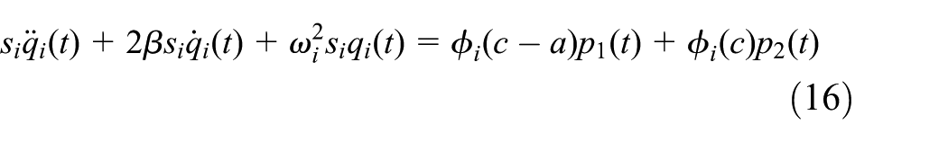
By comparing and analyzing the motion state of each degree of freedom in the vehicle model of Stage II and Stage III, the motion equation of front wheel is the same as equation (11a); the vertical motion and vehicle equation of the body mass can be expressed by the same equations as in Stage II, which are equations (12a) and (12b). While the bridge is not in contact with the rear wheel in Stage II, it is in contact in Stage III, which causes the motion equation of the rear wheel obviously different in Stage II and Stage III. The equation of motion for rear wheel mass $m_{t2}$ is expanded as follows

$$\begin{array}{c}\multicolumn{1}{c}{m_{t2}{\stackrel{··}{y}}_{t2}+c_{a2}({\stackrel{·}{y}}_{t2}-{\stackrel{·}{y}}_2)+k_{a2}(y_{t2}-y_2)+c_{t2}({\stackrel{·}{y}}_{t2}-{\stackrel{·}{y}}_b}\\ \multicolumn{1}{c}{-r_2\stackrel{·}{\theta })+k_{t2}(y_{t2}-y_b-r_2\theta )=m_{t2}g}\end{array}$$

(17)

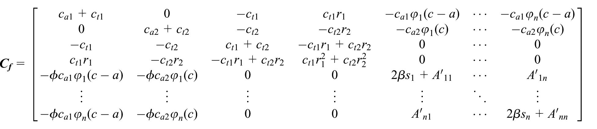
Combining equations (15)–(17), representing the generalized motion equation for the third-stage of vehicle–bridge coupled system in matrix form, yields

$${\mathit{M}}_{\mathit{f}}\stackrel{··}{\mathit{u}}+{\mathit{C}}_{\mathit{f}}\stackrel{·}{\mathit{u}}+{\mathit{K}}_{\mathit{f}}\mathit{u}={\mathit{F}}_{\mathit{f}}$$

(18)

where the elements in ${\mathit{M}}_{\mathit{f}}$ , ${\mathit{F}}_{\mathit{f}}$ are exactly the same as those in ${\mathit{M}}_{\mathit{p}}$ , ${\mathit{F}}_{\mathit{p}}$ in equation (13) and

$$\begin{array}{c}{A\prime }_{\mathrm{ij}}=\phi c_{a1}{\varphi }_i(c-a){\varphi }_j(c-a)+\phi c_{a2}{\varphi }_i(c){\varphi }_j(c)\hfill \\ {B\prime }_{\mathrm{ij}}=\phi k_{a1}{\varphi }_i(c-a){\varphi }_j(c-a)+\phi k_{a2}{\varphi }_i(c){\varphi }_j(c)\hfill \end{array}$$

$${\mathit{C}}_{\mathit{f}}=\left[\begin{array}{ccccccc}{c}_{a1}+c_{t1}\hfill & 0\hfill & -c_{t1}\hfill & c_{t1}{r}_1\hfill & -c_{a1}{\phi }_1(c-a)\hfill & \cdots \hfill & -c_{a1}{\phi }_n(c-a)\hfill \\ \multicolumn{1}{c}{0}& c_{a2}+c_{t2}\hfill & -c_{t2}\hfill & -c_{t2}{r}_2\hfill & -c_{a2}{\phi }_1(c)\hfill & \cdots \hfill & -c_{a2}{\phi }_n(c)\hfill \\ \multicolumn{1}{c}{-c_{t1}}& -c_{t2}\hfill & c_{t1}+c_{t2}\hfill & -c_{t1}{r}_1+c_{t2}{r}_2\hfill & 0\hfill & \cdots \hfill & 0\hfill \\ \multicolumn{1}{c}{c_{t1}{r}_1}& -c_{t2}{r}_2\hfill & -c_{t1}{r}_1+c_{t2}{r}_2\hfill & c_{t1}{r}_1^2+c_{t2}{r}_2^2\hfill & 0\hfill & \cdots \hfill & 0\hfill \\ \multicolumn{1}{c}{-\varphi c_{a1}{\phi }_1(c-a)}& -\varphi c_{a2}{\phi }_1(c)\hfill & 0\hfill & 0\hfill & 2\beta s_1+{A\prime }_{11}\hfill & \cdots \hfill & {A\prime }_{1n}\hfill \\ \multicolumn{1}{c}{⋮}& ⋮\hfill & ⋮\hfill & ⋮\hfill & ⋮\hfill & \ddots \hfill & ⋮\hfill \\ \multicolumn{1}{c}{-\varphi c_{a1}{\phi }_n(c-a)}& -\varphi c_{a2}{\phi }_n(c)\hfill & 0\hfill & 0\hfill & {A\prime }_{n1}\hfill & \cdots \hfill & 2\beta s_n+{A\prime }_{\mathrm{nn}}\hfill \end{array}\right]$$

$${\mathit{K}}_{\mathit{f}}=\left[\begin{array}{ccccccc}{k}_{a1}+k_{t1}\hfill & 0\hfill & -k_{t1}\hfill & k_{t1}{r}_1\hfill & -k_{a1}{\phi }_1(c-a)\hfill & \cdots \hfill & -k_{a1}{\phi }_n(c-a)\hfill \\ \multicolumn{1}{c}{0}& k_{a2}+k_{t2}\hfill & -k_{t2}\hfill & -k_{t2}{r}_2\hfill & -k_{a2}{\phi }_1(c)\hfill & \cdots \hfill & -k_{a2}{\phi }_n(c)\hfill \\ \multicolumn{1}{c}{-k_{t1}}& -k_{t2}\hfill & k_{t1}+k_{t2}\hfill & -k_{t1}{r}_1+k_{t2}{r}_2\hfill & 0\hfill & \cdots \hfill & 0\hfill \\ \multicolumn{1}{c}{k_{t1}{r}_1}& -k_{t2}{r}_2\hfill & -k_{t1}{r}_1+k_{t2}{r}_2\hfill & k_{t1}{r}_1^2+k_{t2}{r}_2^2\hfill & 0\hfill & \cdots \hfill & 0\hfill \\ \multicolumn{1}{c}{-\varphi k_{a1}{\phi }_1(c-a)}& -\varphi k_{a2}{\phi }_1(c)\hfill & 0\hfill & 0\hfill & {\omega }_1^2{s}_1+{B\prime }_{11}\hfill & \cdots \hfill & {B\prime }_{1n}\hfill \\ \multicolumn{1}{c}{⋮}& ⋮\hfill & ⋮\hfill & ⋮\hfill & ⋮\hfill & \ddots \hfill & ⋮\hfill \\ \multicolumn{1}{c}{-\varphi k_{a1}{\phi }_n(c-a)}& -\varphi k_{a2}{\phi }_n(c)\hfill & 0\hfill & 0\hfill & {B\prime }_{n1}\hfill & \cdots \hfill & {\omega }_n^2{s}_n+{B\prime }_{\mathrm{nn}}\hfill \end{array}\right]$$

Equation (18) can be solved for u through substituting the initial conditions in section “Vehicle–bridge coupling vibration equation of Stage II,” then the bridge dynamic displacement time–history curve $y(x,t)$ after vehicle bump could be derived.

Solution of dynamic response

The numerical methods are widely adopted to solve the vehicle–bridge-coupled vibration problem, which include Runge–Kutta method, Wilson-θ method, and Newmark-β method.^21,22 In this article, the fourth-order Runge–Kutta method^28,29 is selected to solve the dynamic response. As for dynamic response of the whole vehicle bump test process, it is easy to solve using the Runge–Kutta method after determining the vehicle–bridge coupling vibration equations in each stage, difficulty of which is how to determine the starting time and initial condition of each stage.

In Stage I, the vehicle–bridge coupling system is in a static equilibrium state. The bridge structure and the 4 degrees of freedom of vehicle have only initial displacements, which can be easily determined by equations (4) and (5), respectively. In this case, the vehicle deformation and bridge deformation are independent of the duration of Stage I, so the initial moment of Stage II has no effect on the solution of the displacement dynamic response, and the starting moment can be given arbitrarily. Therefore, the deformation of each degree of freedom obtained in Stage I is referred to as the initial condition of each degree of freedom of the vehicle model in the second stage, which has

$$y(x,0)\approx \sum _{i=1}^n{\varphi }_i(x)q_i(0)$$

(19)

Multiplying by ${\varphi }_i(x)$ on the left and right sides of equation (19), integrating x between 0 and l at the moment t = 0, yields

$$\underset{0}{\overset{l}{\int }}{\varphi }_i(x)y(x,0)\mathrm{dx}=\underset{0}{\overset{l}{\int }}{\varphi }_i^2(x)q_i(0)\mathrm{dx}$$

(20)

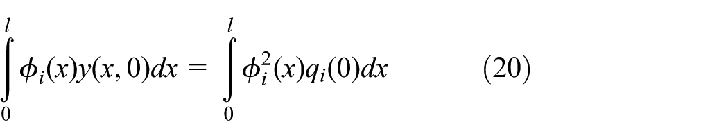
According to equation (20), it has

$$q_i(0)=\frac{{\int }_0^l{\varphi }_i(x)q_i(0)\mathrm{dx}}{{\int }_0^l{\varphi }_i^2(x)\mathrm{dx}}$$

(21)

The value of the modal coordinates of the bridge structure in the first stage in equation (21) is also the modal coordinate and initial value of the bridge in Stage II. As a result, the initial conditions of Stage II are determined by equations (5) and (21).

After determining the initial conditions of Stage II, Runge–Kutta method could be adopted to solve the vehicle–bridge-coupled vibration (equation (13)). In solving the equation, it can be found that there is a time when the displacement of rear wheel is equal to that of the bridge, then this moment could be considered as the time when the rear wheel is in full contact with the bridge structure, which has

$$y_{t2}=y_2$$

(22)

Therefore, this moment is the beginning of Stage III and the obtained $\{u\}$ , $\{\stackrel{·}{u}\}$ , $\{\stackrel{··}{u}\}$ in Stage II is the initial condition of Stage III. After the initial time and initial conditions of Stage III are determined, the vehicle–bridge-coupled vibration equation of Stage III can be solved based on Runge–Kutta method.

By estimating the static deformation of the first-stage and the dynamic response of Stages II and III, the solution of the dynamic response of the whole process of the vehicle bump test is realized.

Field test and numerical calculation

Application to a real structure

The proposed method was applied to an actual project to validate the reliability of the method. PhD Longlin Wang of Guangxi Transportation Research and Consulting Co., Ltd, carried out a load test (including static and dynamic load test) on the Julonghe Bridge to evaluate its operation performance and service condition. The Julonghe Bridge is a simply supported reinforced concrete hollow slab bridge with spans 7 m × 16 m, which is composed of 11 slabs. Its bridge deck is equipped with reinforced concrete pavement. Figures 6–8 represent the general layout and cross section of the Julonghe Bridge, Young’s modulus of which is 3.25 × 10¹⁰ Pa and density is 2600 kg/m³.

Figure 6.

The general layout of the Julonghe Bridge (unit: cm).

Figure 7.

The cross section of the Julonghe Bridge (unit: cm).

Figure 8.

The cross section of the hollow slab (unit: cm).

The 1# and 2# spans of the test bridge were selected to perform the load test. In the vehicle bump test of dynamic load test, two obstacles with height of 15 cm were placed at the mid-span of 2# test span. The left and right obstacles were placed at 0.6 and 2.4 m from the left guardrail as the lateral width of test vehicle is 1.8 m. Let the front axle of the three-axle test vehicle move to the top of obstacles very slowly and then brake immediately (Figure 9). It is obvious from Figure 10 that the test data measured by strain sensors are collected through the strain acquisition system; the strain values of each measuring point at the monitoring cross section in vehicle bump test are obtained. “▮” in Figure 6 represents the strain monitoring cross section and “▬” arranged at the underside of the hollow slab in Figure 7 stands for the strain monitoring point.

Figure 9.

The field test.

Figure 10.

Strain sensors.

A three-axle vehicle in Figure 9 is adopted as the test vehicle in this field test, which is simplified as a planar model provided in Figure 11 and the vehicle parameters measured in practice are shown in Table 1.

Figure 11.

The three-axle test vehicle model.

Table 1.

List of the vehicle parameters measured in practice.

Parameters	Value	Parameters	Value
$m_{t1}(\mathrm{kg})$	$3.595\times {10}^2$	$c_{a1}(\mathrm{N}·\mathrm{s}/\mathrm{m})$	6 × 103
$m_{t2}(\mathrm{kg})$	$5.955\times {10}^2$	$c_{a2}(\mathrm{N}·\mathrm{s}/\mathrm{m})$	1.2 × 104
$m_{t3}(\mathrm{kg})$	$5.425\times {10}^2$	$c_{a3}(\mathrm{N}·\mathrm{s}/\mathrm{m})$	1.2 × 104
$m_b(\mathrm{kg})$	3.45 × 104	$k_{t1}(\mathrm{N}/\mathrm{m})$	1.2 × 106
$I_b(\mathrm{kg}·{\mathrm{m}}^2)$	1.2 × 105	$k_{t2}(\mathrm{N}/\mathrm{m})$	2.4 × 106
$k_{a1}(\mathrm{N}/\mathrm{m})$	2.4 × 106	$k_{t3}(\mathrm{N}/\mathrm{m})$	2.4 × 106
$k_{a2}(\mathrm{N}/\mathrm{m})$	4.4 × 106	$c_{t1}(\mathrm{N}·\mathrm{s}/\mathrm{m})$	5 × 103
$k_{a3}(\mathrm{N}/\mathrm{m})$	4.4 × 106	$c_{t2}(\mathrm{N}·\mathrm{s}/\mathrm{m})$	1 × 104
$L_1,L_2(\mathrm{m})$	3.6, 1.4	$c_{t3}(\mathrm{N}·\mathrm{s}/\mathrm{m})$	1 × 104

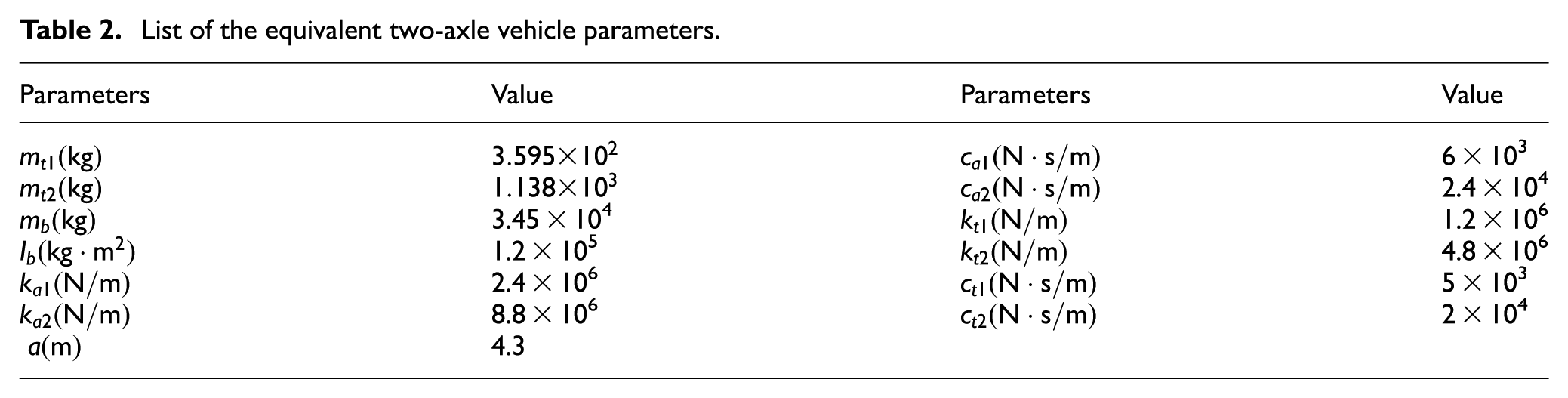
In order to calculate the strain values of monitoring points at the mid-span by the proposed method, the three-axle test vehicle adopted in the field test is needed to be simplified as that of the two-axle test vehicle with 4 degrees of freedom as described in Figure 12. In this vehicle bump test, the front axle was placed at the obstacles with height of 15 cm, and at this time, the suspended height of middle axle is about 4.1 cm, however, considering that the elongation of suspension spring under the axle load is larger than the suspended value. The middle axle and the rear axle of the three-axle vehicle are in contact with the bridge deck which is consistent with the vehicle conditions in the field test. Therefore, the middle axle and the rear axle of the three-axle vehicle could be equivalent to the rear axle of the two-axle one. The equivalent two-axle vehicle parameters are shown in Table 2.

Figure 12.

The equivalent two-axle test vehicle model.

Table 2.

List of the equivalent two-axle vehicle parameters.

Parameters	Value	Parameters	Value
$m_{t1}(\mathrm{kg})$	$3.595\times {10}^2$	$c_{a1}(\mathrm{N}·\mathrm{s}/\mathrm{m})$	6 × 103
$m_{t2}(\mathrm{kg})$	$1.138\times {10}^3$	$c_{a2}(\mathrm{N}·\mathrm{s}/\mathrm{m})$	2.4 × 104
$m_b(\mathrm{kg})$	3.45 × 104	$k_{t1}(\mathrm{N}/\mathrm{m})$	1.2 × 106
$I_b(\mathrm{kg}·{\mathrm{m}}^2)$	1.2 × 105	$k_{t2}(\mathrm{N}/\mathrm{m})$	4.8 × 106
$k_{a1}(\mathrm{N}/\mathrm{m})$	2.4 × 106	$c_{t1}(\mathrm{N}·\mathrm{s}/\mathrm{m})$	5 × 103
$k_{a2}(\mathrm{N}/\mathrm{m})$	8.8 × 106	$c_{t2}(\mathrm{N}·\mathrm{s}/\mathrm{m})$	2 × 104
$a(\mathrm{m})$	4.3

Using this method, the displacement time–history response of each beam at any position in the vehicle bump test can be calculated. If the displacement response of the beam at t_i time is y (x, t_i), then the curvature k of the beam can be defined as follows

$$k=-\frac{d^{2}y(x,t_i)}{d{x}^2}$$

(23)

Then, the strain response at any position is calculated by

$$\epsilon (x,t_i)=k{y}_z=-y_z\frac{d^{2}y(x,t_i)}{d{x}^2}$$

(24)

where $y_z$ represents the distance from monitoring point to the neutral axis.

The strain time–history curve of monitoring points at the mid-span of 2# test span is calculated according to the method proposed in this article. The strain time–history curves of 1# and 3# slabs at the mid-span of 2# test span are derived by the proposed method and field test in order to compare the results of these two methods, which can be observed in Figures 13 and 14.

Figure 13.

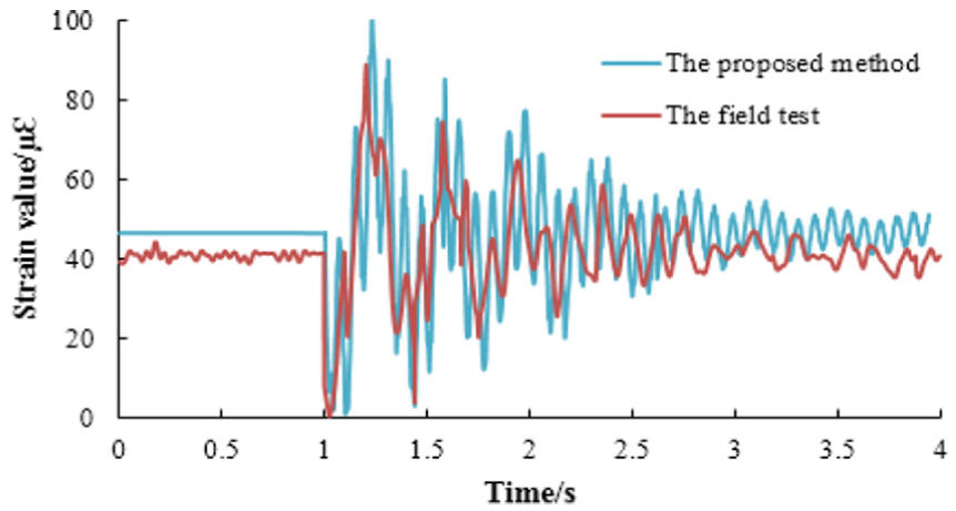
The strain time–history curves of 1# slab at the mid-span of 2# test span.

Figure 14.

The strain time–history curves of 3# slab at the mid-span of 2# test span.

It can be seen in Figures 13 and 14 that the variation trends of strain time–history curves of 1# and 3# slabs have a good agreement. The calculated results of two strain time–history curves are close to the field test, errors of which at the maximum strain values are 12.36% and 12.89%, respectively. These phenomena also validate that the proposed method in this article possesses reliability. Through the analysis of calculation model, it could be found that the reasons for the error between these two results are as follows: (1) the test vehicle adopted in the field test is three-axle vehicle; however, the three-axle vehicle is equivalent to a two-axle one when the proposed method is employed to calculate the strain time–history curve; (2) the bridge deck of the test bridge is equipped with reinforced concrete pavement, existence of which leads to the calculation error of the transverse distribution coefficient of the test bridge; and (3) there is some test error caused by environmental factors in the process of field test.

Numerical example

An actual uniform simply supported T-shaped bridge of 20 m with five girders is numerically simulated. Figures 15 and 16 illustrate the general layout and cross section of the T-shaped bridge. As it can be seen, numbers 1–5 under girders represent the numberings of main girders. The parameters are as follows: Young’s modulus is 3.25 × 10¹⁰ Pa and density is 2500 kg/m³. Since the vehicle model in the work by Mulcahy ³⁵ is used in most of the bridge detections, as a result, it is also adopted in this section and its lateral width is 1.8 m. The mass of vehicle body is usually adjusted as about 36,000 kg in line with practical engineering experience, so 36,000 kg is chosen in this article. The eccentric compression method is selected in this numerical example.

Figure 15.

The general layout of the T-shaped bridge (unit: cm).

Figure 16.

The cross section (unit: mm).

As can be seen in Figure 15, the transverse position of vehicle bump at the mid-span of 1# beam is presented. The mid-span displacement responses of 1# beam are calculated at different heights of vehicle bump, which are shown in Figure 17.

Figure 17.

The displacement responses.

Using the following equation, the bending moment of any cross section at any moment can be calculated

$$M(t_i,x)=\mathrm{EI}\frac{d^{2}y(t_i,x)}{d{x}^2}$$

(25)

Then, the corresponding maximum bending moment are derived when the bump heights are 0, 5, 10, 15, 20, 23 cm, respectively, and the calculation results are exhibited in Figure 18.

Figure 18.

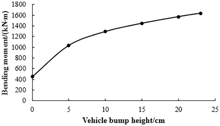
The correlation between vehicle bump heights and bending moments.

It is obvious from Figure 18 that the bending moment increases with the increase in the bump height, and the variation between the bump height and the bending moment is nonlinear.

The maximum moment in the mid-span of the 1# beam reaches the design moment value 1636.39 kN m with the bump height of 23 cm, which can be considered to be the limit bump height at the mid-span of 1# girder of the simply supported bridge. In the case of limit bump height, the displacements of each point of each girder are provided in Figure 19. Correspondingly, the bending moments of each girder are shown in Figure 20.

Figure 19.

The displacements at the moment when the displacement in mid-span is maximum.

Figure 20.

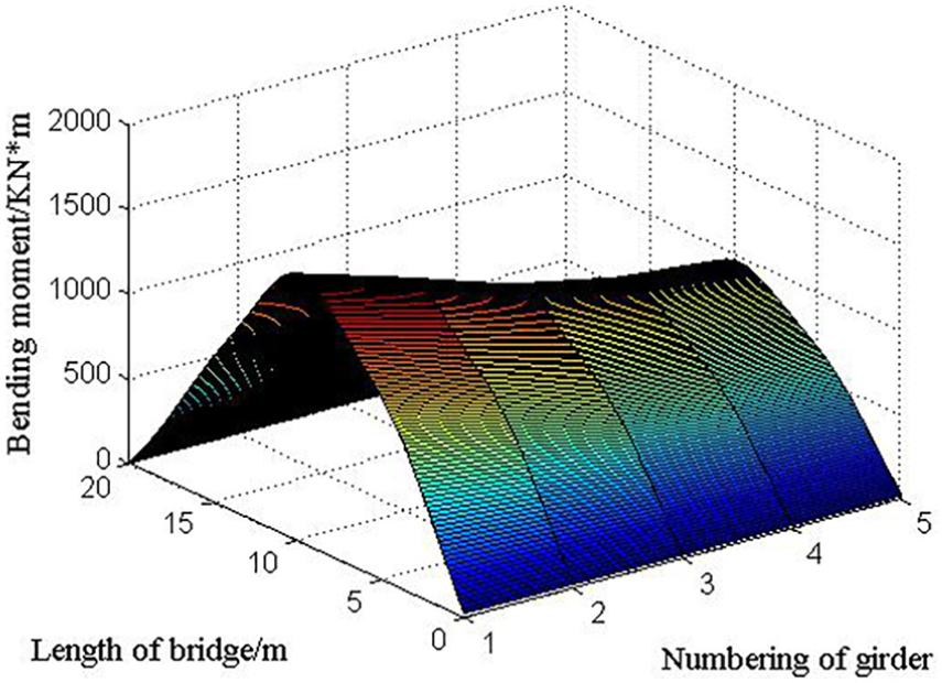
The bending moment when the bending moment of mid-span is maximum.

As can be observed in Figures 19 and 20, when the vehicle bump takes place at the mid-span of 1# girder with limit height, the maximum displacement and bending moment of mid-span lie in 1# girder, which reveals that the 1# girder excitation effect is the most apparent and there is a stronger dynamic response. The further away from the bump position, the smaller the dynamic response of the other beams, which is consistent with the change of load transverse distribution coefficient of simply supported beams.

The displacement responses of the vehicle system in Stage II with various degrees of freedom are derived in this article. When the limit bump height is determined in the above case, the displacement responses of rear wheels in Stage II and the contact point at the mid-span of bridge deck can be obtained, as shown in Figure 21.

Figure 21.

The displacement response of rear wheel in Stage II and contact point at the mid-span of bridge deck.

It is apparent from Figure 21 that the displacement coordinate difference of rear wheel and the bridge is less than 0.0001 m at 0.188 s which could be considered as a contact between both of them. Therefore, it can be concluded that 0.188 s is the initial time of Stage III.

When the height of vehicle bump reaches the limit value, the displacement response of mid-span in 1# girder is shown in Figure 22, from which the displacement response in the whole process can be seen.

Figure 22.

The displacement response in the whole process of mid-span at limit height of vehicle bump.

Conclusion

The theoretical research on the whole process dynamic response solution of bridge structure in vehicle bump test is carried out in this article. The feasible and effective calculation model and estimation method are formed. Then, a field test is conducted to verify the reliability of the method. The dynamic response of considering the transverse position of vehicle bump is calculated based on the numerical simulation of a T-shaped simply supported beam bridge. Finally, we can arrive at the following conclusions:

1. The method proposed in this article divides the vehicle bump test into three stages, so that it can calculate the full-process dynamic response of a vehicle falling from an obstacle. Therefore, the proposed method is different from the vibration analysis considering pavement roughness, which is the biggest innovation of this article.

2. It can be seen from the numerical simulation of T-shaped beam that the initial condition of Stage III is crucial to the method proposed in this article.

3. The strain time–history curves calculated by the proposed method are quite close to that of the field test. The errors at the maximum strain values of these two results are less than 15%, which illustrate that the proposed method possesses reliability and could be applied to practical engineering.

4. When the vehicle bump height is certain, the dynamic response of a simply supported bridge with multiple girders is related to the load transverse distribution coefficient. The larger the transverse distribution coefficient is, the greater the dynamic response is.

5. The bending moment increases with the increase in the bump height, and the correlation between the vehicle bump heights and the bending moments is nonlinear.