Sage Journals: Discover world-class research

Abstract

The steel-concrete composite girder bridge is a new type of bridge. The steel girder and concrete slab are connected together by connectors and bear the common force so that the tensile performance of steel and the compressive performance of concrete can be fully utilized. The advantages are obvious. However, research on the dynamic analysis of steel-concrete composite beam bridges is still relatively rare, and the dynamic effects on these bridges from vehicles are becoming increasingly significant. In this paper, a more complex steel-concrete composite simply supported beam bridge model and the entire vehicle model are established, and five steel-concrete connection levels of the bridge model are considered. Using the finite element model, the effects of five factors, namely, bridge natural frequency, vehicle natural frequency, vehicle speed, vehicle lateral position and bridge deck roughness, on the dynamic load allowance (DLA) of the composite girder bridge are studied. The influence of vehicle speed and bridge surface roughness on the DLA has a strong regularity. The change in the DLA of the lateral position of the vehicle is highly symmetrical, and the DLA value at the side beam is larger than that of the center beam. Changes in bridge vibration frequency and vehicle vibration frequency can bring about significant changes in the DLA, and the closer the two frequencies are, the more significant the DLA increases, and the more likely it is to produce resonance.

Keywords

Steel-concrete girder bridges vehicle-bridge coupled vibration dynamic responses interface slip

Introduction

In recent years, more than 878,300 highway bridges have been built in China. In terms of the number of bridges and the span of various types of bridges, China has become the world’s largest bridge country. However, the development of bridges in China has been extremely uneven. Concrete bridges account for the vast majority, while steel bridges and composite beam bridges account for a very small proportion with steel-concrete composite beam bridges accounting for less than 1%. In some traditional bridge authorities, steel-concrete composite beam bridges have been widely used. Comparing these bridge authorities, China should gradually improve the status quo of this uneven bridge development. In addition, with the increasing downward pressure on China’s economy, the overcapacity of steel has become serious, directly endangering the healthy development of the industry and the national economy. Bridge practitioners should speed up research on bridge forms and accelerate the promotion and application of steel bridges and steel-concrete composite bridges. The proportion of structural steel in long-span bridges is relatively large. However, in China, most of the small- and medium-span bridges are concrete bridges, so the focus is on improving these types of bridges. The steel structure is not suitable for small and medium-span bridges as steel structure low rigidity and high vibration can easily lead to fatigue problems. Therefore, steel-concrete composite beam bridges have become the best choice for small and medium-span bridges. The steel-concrete composite beam bridge can fully exploit the advantages of steel and concrete so that the tensile performance of steel and the compressive performance of concrete can be fully exploited. Steel, which can be economical and environmentally friendly, has clear advantages in medium- and small-span bridges.^1,2

The steel beam and the concrete slab of the steel-concrete composite beam bridge are connected by shear connectors.^3–6 During long-term use, the steel-concrete composite girder bridge is under repeated load fatigue,^7,8 and under the impact of dynamic load^9,10 the shear connectors will gradually be destroyed, resulting in slippage which reduces the connection performance of the composite structure. The overall stiffness decreases, the bearing capacity decreases, and the natural vibration performance of the structure changes. The steel-concrete composite girder bridge will inevitably slip between the steel girder and the concrete over time, with a major impact on the long-term performance of the bridge. It is important to ensure effective connection in the steel-concrete composite. The safety of the beam bridge is critically important.¹¹ Vehicle load movement is the main form of load during the operation of highway bridge structures. Nearly 40% of bridge damage is caused by the vibration of moving vehicles. Therefore, the design of steel-concrete composite beam bridges necessitates further requirements to be put forward to improve the dynamic performance.

Previous studies have shown that the interface slip effect of the steel-concrete composite beam bridge has a certain impact on the dynamic performance of the composite beam bridge. As interface slip occurs, the overall stiffness of the composite beam decreases, and the natural frequency of the composite beam decreases.^12–14 The influence of multiple factors such as interface slip, shear deformation and moment of inertia are considered to study the natural vibration characteristics of steel-concrete composite truss beam.¹⁵ Most of the previous studies have focused on the free vibration of the structure and have not conducted much investigation into the bridge natural vibration performance under moving loads; the simulation of the vehicle load in the literature is relatively simple, and the literature considering the coupled vibration of the vehicle and bridge is rare.^15–20

For railway bridge, there are some research results. Liu et al. proposes a theoretical method of calculating the train-induced vibration and noise of a constrained layer damping-enhanced railway bridge based on the train-track-bridge coupled vibration, the modal strain energy method, and statistical energy analysis.²¹ Szurgott and Bernacki proposes a method for modeling and simulating the transient vibrations of a system comprising a steel-concrete bridge, ballasted track and moving high-speed train. The proposed approach uses advanced LS-DYNA simulation software based on finite element (FE) analysis and is applied to a series of single-span simply supported steel-concrete bridges.²² To evaluate how the inclusion of local deck vibrations might influence predictions of the maximum acceleration, detailed measurements are taken from a steel-concrete composite box-girder bridge on the Italian high-speed railway, and a numerical model of the system is developed.²³ For monorail bridges, a new finite element model of steel-concrete composite beam which can simulate the slip phenomenon is proposed.²⁴ The dynamic response of under-deck cable-stayed bridges with steel-concrete composite decks under moving loads is presented, and different parameters are considered.²⁵

As we know, the phenomenon of vehicle-bridge coupled vibration is common in highway bridge, especially for small- and medium-span beam bridges. However, some large span bridges are much more focused on.^26–31 There are fewer studies that have considered the important influencing factor of road surface roughness, and there are few studies on the dynamic performance of continuous steel-concrete composite beam bridges under moving loads. Therefore, there is an urgent need for research in this area.

It is necessary to study the dynamic performance of the steel-concrete composite beam bridge under moving vehicle loads. Using the Jingha Expressway overpass, this paper establishes a vehicle-bridge vibration simulation model of steel-concrete composite girder bridges with different connection levels. The established vehicle model considers the coupled vibration of the vehicle bridge and the unevenness of the bridge deck with systematical analysis. The influence of key factors such as bridge natural frequency, vehicle natural frequency, vehicle speed, vehicle lateral position, and bridge deck unevenness on the dynamic response of steel-concrete composite girder bridges is analyzed.

Vehicle-bridge coupled vibration

When a vehicle is driving on a highway bridge, it causes the bridge to vibrate, thereby affecting the vibration of the vehicle.³² This interaction and influence represent the coupled vibration between the vehicle and the bridge. From the perspective of dynamics, a car is a multi-degree-of-freedom vibration system composed of a car body, wheels and suspension system. Due to the weight of the vehicle and the unevenness of the bridge deck, the moving vehicle has a dynamic impact on the bridge structure, forcing the bridge to vibrate, which in turn affects the vibration of the vehicle. In this way, the vehicle and the bridge influence each other through the contact between the wheels and the bridge deck, thereby forming a complex multi-degree-of-freedom coupled vibration system.^33,34

Theoretical vehicle-bridge coupled vibration calculations first require numerical model expressions of factors such as vehicle structure, bridge structure and road surface roughness. In terms of model research, vehicle motion mainly includes pitching, ups and downs, and rollover of the vehicle body. Vehicle models are usually established based on the Hamilton principle or d’Alembert principle. Bridge model construction methods mainly include the modal coordinate method and finite element method. With the development of computer technology, the finite element method is widely used because of its high calculation accuracy and fast modeling speed. For simulating bridge surface roughness, the main generation methods are the time series method, white noise excitation simulation method, type analysis method, inverse Fourier transform method, and trigonometric series method. A reasonable vehicle model, bridge model, and bridge surface roughness model are then established. After separating the bridge and the vehicle into a multi-node finite element model, the coupled vibration equation of the bridge and the vehicle can be established as follows:

[M_{b}] {\overset{\cdot\cdot}{y}} + [C_{b}] {\overset{\cdot}{y}} + [K_{b}] {y} = {F_{vb}}

[M_{v}] {\overset{\cdot\cdot}{z}} + [C_{v}] {\overset{\cdot}{z}} + [K_{v}] {z} = {F_{bv}} + {F_{vg}}

where [M], [C], [K] are the mass matrix, damping matrix and stiffness matrix, respectively. Subscripts v and b represent vehicles and bridges, respectively. {y} and {z} are the displacement vectors of the bridge and vehicle system nodes. {F_vg} is the equivalent value caused by the nodal load sequence vector of the vehicle’s own weight. {F_vb} and {F_bv} are the interactions of the tire-bridge contact points obtained by the shape function distribution, respectively. The nodal load vector of the force is where the vehicle-bridge contact force is a function of the bridge, the vehicle displacement, and the road surface roughness at the contact point.²⁰

The vehicle-bridge coupled vibration equation is a nonlinear time-varying equation. The load response of vehicles and bridges can be obtained by the modal synthesis and direct integration methods. The direct integration method is commonly used to solve such problems, mainly including the Wilson-θ method, the Newmark-β method, the Runge-Kutta method, and other numerical integration methods. Such a simulation system can effectively simulate bridge vibrations of different vehicle types, different vehicle speeds, different road smoothness, and different bridge types and structural sizes to obtain a complete time history response of bridge and vehicle vibration during the entire process of vehicles passing the bridge.

Numerical simulation

Sample selection of the steel-concrete composite simply supported girder bridge

There are quite a few types of steel-concrete composite beam bridges, including T-shaped steel-concrete composite beam bridges, box-section steel web composite beam bridges, corrugated steel web composite beam bridges, and channel steel-concrete composite beam bridges. Among them, T-shaped steel-concrete composite beam bridges are the most common. Considering flange slab construction technology, they can be divided into precast concrete flange slabs, cast-in-place concrete flange slabs, profiled steel flange slabs, and laminated flange slabs. This paper studies a small- and medium-span T-shaped steel-concrete composite simple-supported beam bridge with a cast-in-place concrete flange slab.

The example bridge selected in this paper is a viaduct in the Beijing-Harbin Expressway. The bridge is a steel-concrete composite girder bridge with a longitudinal length of 30 m and a lateral width of 8 m. A schematic diagram of the cross-section is shown in Figure 1. Three girders are set transversely, adopting an I-cross section, and the spacing between the girders is 2.4 m. The steel girder and concrete slab are connected by studs.

Figure 1.

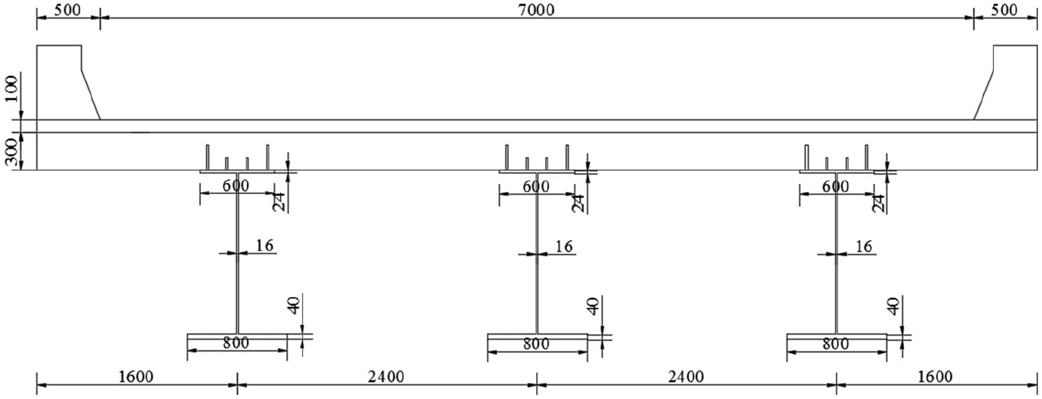
Cross section of the girder (mm).

ANSYS finite element analysis software is used to establish the solid-shell finite element model following the cross-sectional dimensions and material properties of the composite beam bridge drawing. The concrete slab is made of C50 concrete, with a Young’s modulus of 3.45 × 10⁴ MPa. It is simulated by the Solid65 element in the ANSYS finite element analysis software. The steel girder is made of Q345 steel, with a Young’s modulus of 2.06 × 10⁵ MPa. It is simulated by the Shell181 unit in the ANSYS finite element analysis software. The Combin39 unit is used for the shear connection. For concrete slabs, there are 4650 nodes and 2700 elements. For steel girders, there are 6045 nodes and 450 elements. The established finite element model is shown in Figure 2.

Figure 2.

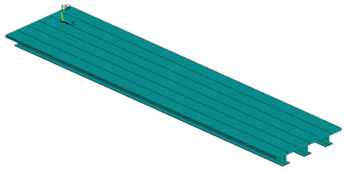
Finite element model.

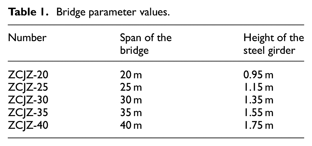
The bridge frequency of the T-shaped steel-concrete composite simple-supported girder bridge is controlled by the parameters of the bridge span and the steel girder height. The original bridge span is 30 m, so the five bridge spans that we selected are 20 m, 25 m, 30 m, 35 m, and 40 m. The steel girder height of the original viaduct is 1.35 m, so the heights of the five steel girders that we selected are 0.95 m, 1.15 m, 1.35 m, 1.55 m, and 1.75 m. The bridge parameter values are given in Table 1.

Table 1.

Bridge parameter values.

Number	Span of thebridge	Height of thesteel girder
ZCJZ-20	20 m	0.95 m
ZCJZ-25	25 m	1.15 m
ZCJZ-30	30 m	1.35 m
ZCJZ-35	35 m	1.55 m
ZCJZ-40	40 m	1.75 m

As we know, for simply supported beam bridge, the first four mode shapes are similar for bridges with different span length. Therefore, mode shapes of the 30 m-span bridge are shown in Figure 3.

Figure 3.

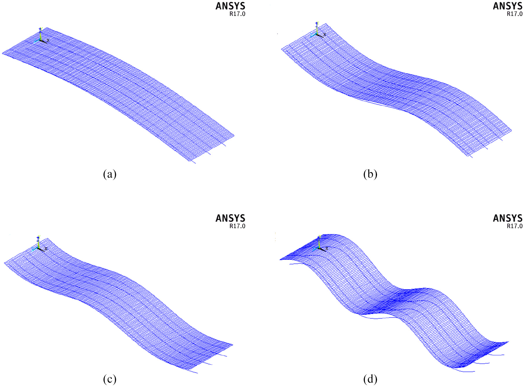
Mode shapes obtained by program ANSYS: (a) 1st mode shape, (b) 2nd mode shape, (c) 3rd mode shape, and (d) 4th mode shape.

Moving vehicle load parameters

There are many types of vehicles. Taking into account the vertical freedom of the four wheels and that of the rigid body of the vehicle, this paper establishes a four-wheel vehicle model. The distance between the front and rear axles of the vehicle is 3 m, which can basically reflect the actual operating conditions of the vehicle and allow accurately coupling with the bridge model. The original drawing indicates that the vehicle load level of the bridge is Highway-II. According to the information, a vehicle model is established, and the vehicle parameters are determined.

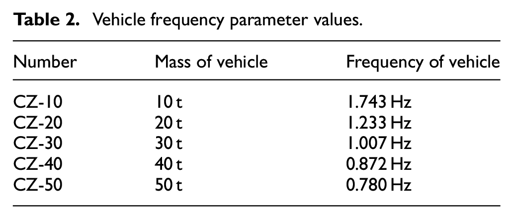
The vehicle frequency is changed by controlling the spring stiffness of the vehicle and changing the vehicle mass parameters. We select vehicle weights of 10 t, 20 t, 30 t, 40 t, and 50 t to calculate the corresponding vehicle frequency. The vehicle frequency parameter values are given in Table 2.

Table 2.

Vehicle frequency parameter values.

Number	Mass of vehicle	Frequency of vehicle
CZ-10	10 t	1.743 Hz
CZ-20	20 t	1.233 Hz
CZ-30	30 t	1.007 Hz
CZ-40	40 t	0.872 Hz
CZ-50	50 t	0.780 Hz

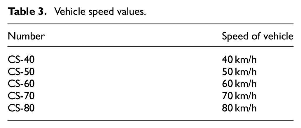
The vehicle load class of this bridge limits the vehicle speeds from 40 km/h to 80 km/h, so we select five vehicle speeds of 40 km/h, 50 km/h, 60 km/h, 70 km/h, and 80 km/h. The vehicle speed parameter values are given in Table 3.

Table 3.

Vehicle speed values.

Number	Speed of vehicle
CS-40	40 km/h
CS-50	50 km/h
CS-60	60 km/h
CS-70	70 km/h
CS-80	80 km/h

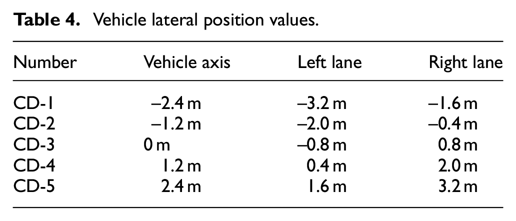
The vehicle lateral position is achieved by controlling the trajectory of the left and right wheels of the vehicle, and the corresponding distances between the vehicle’s central axis and the bridge’s central axis are −2.4 m, −1.2 m, 0 m, 1.2 m, and 2.4 m, respectively. The vehicle lateral position values are given in Table 4.

Table 4.

Vehicle lateral position values.

Number	Vehicle axis	Left lane	Right lane
CD-1	−2.4 m	−3.2 m	−1.6 m
CD-2	−1.2 m	−2.0 m	−0.4 m
CD-3	0 m	−0.8 m	0.8 m
CD-4	1.2 m	0.4 m	2.0 m
CD-5	2.4 m	1.6 m	3.2 m

Simulation of pavement roughness

The pavement roughness is one of the main influencing factors of the bridge’s dynamic responses. The pavement roughness is the most important form of load excitation during the driving process which must be considered in vehicle-bridge coupled vibration analysis.

In this paper, the road surface power spectrum theory is used to simulate the pavement roughness. The theory regards the pavement roughness as a stable and random process with various states, zero mean and Gaussian distribution. In this paper, the irregularity parameters are randomly calculated by compiling the MATLAB program. A series of numbers are obtained through it, which are applied to the bridge deck together as the excitation load and the vehicle load.

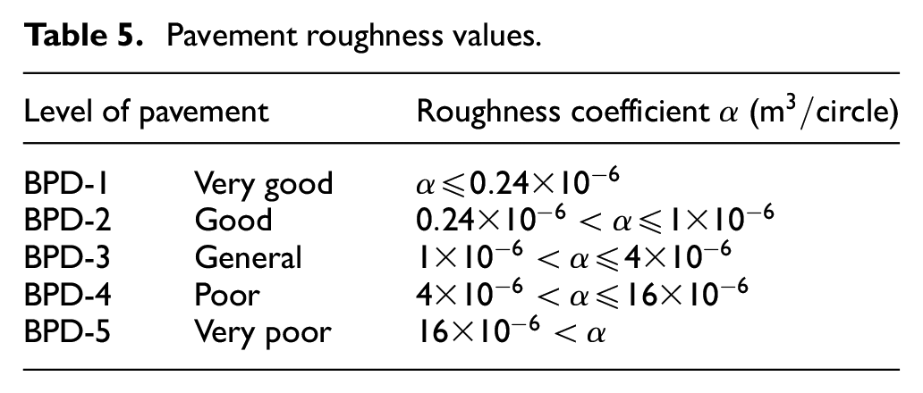
By controlling the upper and lower limits of the effective spatial frequency of the bridge roughness power spectrum density roughness coefficient, the roughness parameters of the left and right lanes are generated, respectively, and five types of uneven bridge samples are obtained. The roughness values are given in Table 5.

Table 5.

Pavement roughness values.

Level of pavement		Roughness coefficient $α (m^{3} / circle)$
BPD-1	Very good	$α \leq 0.24 \times 10^{- 6}$
BPD-2	Good	$0.24 \times 10^{- 6} < α \leq 1 \times 10^{- 6}$
BPD-3	General	$1 \times 10^{- 6} < α \leq 4 \times 10^{- 6}$
BPD-4	Poor	$4 \times 10^{- 6} < α \leq 16 \times 10^{- 6}$
BPD-5	Very poor	$16 \times 10^{- 6} < α$

Classification of interface connection levels between steel girder and concrete slab

This paper divides the interface connection degree between the steel girder and the concrete slab into ten levels. The shear stiffness of the interface connection increases gradually as the connection level increases. The shear stiffnesses of the interface connection in the specific finite element model are given in Table 6.

Table 6.

Classification of interface connection levels.

Connectionlevel	The shearstiffness(kN/m)	Connectionlevel	The shearstiffness(kN/m)
1	9.3 × 10¹	6	9.3 × 10⁶
2	9.3 × 10²	7	9.3 × 10⁷
3	9.3 × 10³	8	9.3 × 10⁸
4	9.3 × 10⁴	9	9.3 × 10⁹
5	9.3 × 10⁵	10	9.3 × 10¹⁰

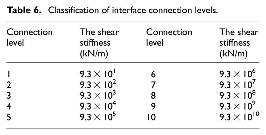
In the composite beam bridge natural frequency calculation, it is found that when the connection level is reduced from 2 to 1, the fundamental frequency of the bridge is reduced from 2.6146 Hz to 2.6143 Hz. When the shear stiffness of the interface connection is continuously reduced, the fundamental frequency of the bridge basically no longer decreases, indicating that the shear connectors of the composite girder bridge have failed and the that bridge has entered a state where the concrete slab and steel girder are superimposed without forming a composite section. When the connection level is increased from 9 to 10, the fundamental frequency of the bridge is increased from 4.0408 Hz to 4.0417 Hz. When the shear stiffness of the interface connection is continuously increased, the fundamental frequency of the bridge basically is no longer increased, meaning that the concrete slab and the steel girder form a whole section and the connection is tight without slippage. If the connection level is sufficiently small or large, the corresponding DLA values are very close.

The five connection levels with more drastic changes include 4, 5, 6, 7, and 8, so we select only these five types of connection levels in this study.

Dynamic responses of concrete slabs

Influence of bridge frequency

A 30t vehicle moves at a constant speed of 60 km/h, and the vehicle travels along the center axis for the full bridge length. The level of the pavement is general at this time, and the parameter values of the bridge are selected according to Table 1. The five connection levels are considered to establish 25 finite element models. Then, we extract the maximum dynamic deflection value of the concrete slab from the finite element model and calculate the maximum static deflection value of the concrete slab in order to determine the DLA.

DLA value of the concrete slab under the influence of the bridge natural frequency are shown in Figure 4.

Figure 4.

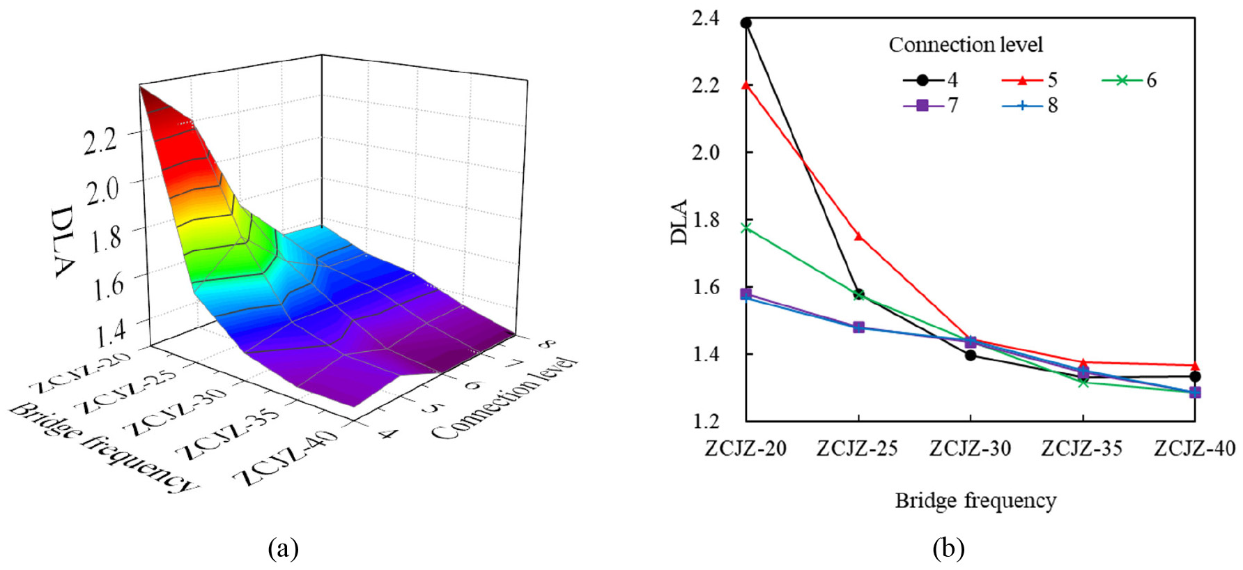
DLA value of the concrete slab under the influence of the bridge natural frequency: (a) 3D plot, and (b) 2D plot.

Figure 4 shows that the DLA of the concrete slab gradually decreases with increasing bridge span and continuously decreases with continuous strengthening of the connection level. The reason is that the mass of the bridge will increase with increasing bridge span and steel beam height, and the vehicle load becomes increasingly small relative to the weight of the bridge. Then, its dynamic effect on the bridge gradually decreases, corresponding to the steadily decreasing DLA.

Influence of vehicle frequency

DLA value of the concrete slab under the influence of vehicle frequency are shown in Figure 5.

Figure 5.

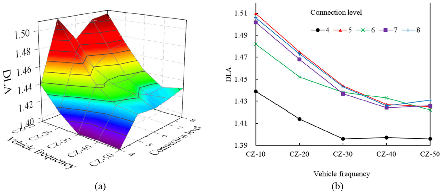
DLA value of the concrete slab under the influence of vehicle frequency: (a) 3D plot and (b) 2D plot.

Figure 5 shows that the DLA of the concrete slab increases rapidly with increasing vehicle frequency, but the change in the connection level has relatively little effect on the DLA of the concrete slab. The reason is that the vehicle load has a significant impact on the dynamic response of the bridge as the main load form during the operation of the bridge, especially for small cars with a high frequency of vehicles.

Influence of vehicle speed

DLA value of the concrete slab under the influence of vehicle speed are shown in Figure 6.

Figure 6.

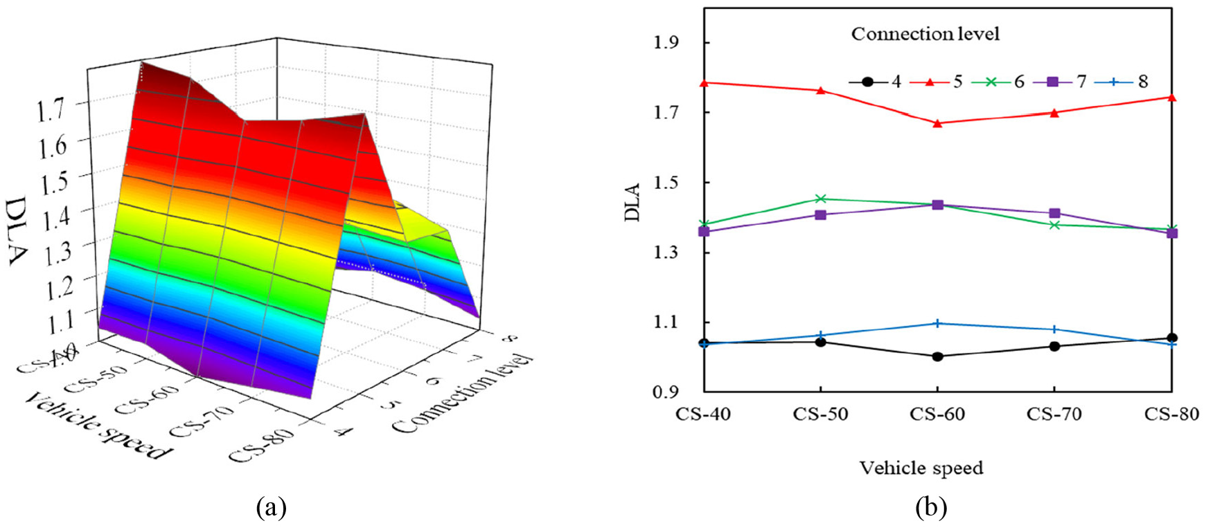
DLA value of the concrete slab under the influence of vehicle speed: (a) 3D plot and (b) 2D plot.

Figure 6 shows that when the connection level is low, the DLA of the concrete slab first decreases and then increases with increasing driving speed. When the connection level is higher, it increases and then decreases as the driving speed increased. The reason is that the impact of vehicle speed on the DLA generally changes in a W-shaped manner. Different connection levels correspond to different peaks and valleys of the W-shaped curve. Therefore, when the connection level is low, the DLA changes in a V-shaped curve with the driving speed. When the connection level is high, it changes in an N-shaped curve with the driving speed.

Influence of vehicle location

DLA value of the concrete slab under the influence of vehicle location are shown in Figure 7.

Figure 7.

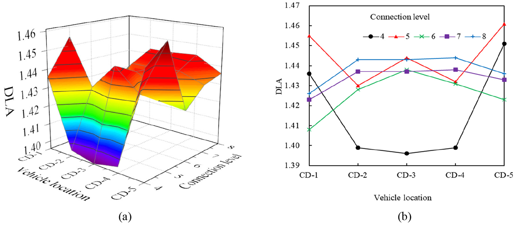
DLA value of the concrete slab under the influence of vehicle location: (a) 3D plot and (b) 2D plot.

Figure 7 shows that the DLA of the concrete slab is distributed very symmetrically in the lateral position, and the dynamic effects generated by vehicle driving on the left and right sides of the bridge are relatively similar. When the connection level is lower, the DLA of the vehicle driving on the side beam is larger. When the connection level is higher, the DLA of the vehicle driving on the center beam is larger. The reason for this phenomenon is that the stiffness of the side beam is smaller than that of the middle beam, so the dynamic effect of the vehicle on the side beam is more obvious. This phenomenon is more apparent when the connection level is lower. The concrete and steel girder are connected as a whole after the connection level becomes larger, so the DLA of the vehicle driving on the center beam is relatively large at this point.

Influence of pavement roughness

DLA value of the concrete slab under the influence of pavement roughness are shown in Figure 8.

Figure 8.

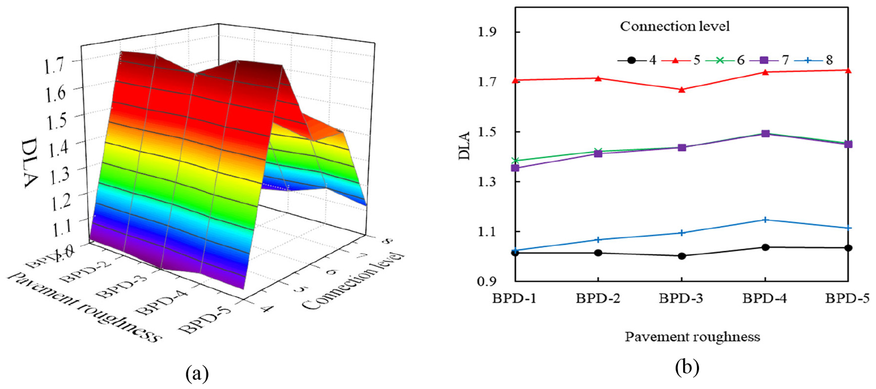
DLA value of the concrete slab under the influence of pavement roughness: (a) 3D plot and (b) 2D plot.

Figure 8 shows that the DLA of the concrete slab increases with increasing roughness coefficient of the pavement, and the DLA first increases and then decreases with increasing connection level. The reason is that the roughness of the pavement is the main load excitation when the vehicle is driving on the bridge, and it has a more obvious impact on the bridge dynamic response. When the roughness coefficient is small, the DLA is small. When the roughness coefficient is large, the DLA is relatively large. In addition, the connection level has a greater impact on the DLA than the pavement roughness.

Dynamic responses of steel girders

Since the DLA of the steel girder calculated by deflection is very close to that of the concrete slab, the DLA value of the concrete slab is given in the previous section. In this section, the DLA value of the steel girder is calculated through stress calculations to compare with that of the concrete slabs.

Influence of bridge frequency

DLA value of the concrete slab and the steel girder under the influence of bridge natural frequency are shown in Figure 9.

Figure 9.

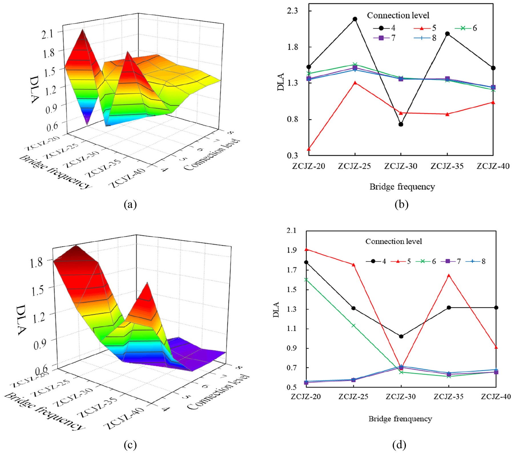
DLA value of the concrete slab and the steel girder under the influence of bridge natural frequency: (a) the concrete slab (3D plot), (b) the concrete slab (2D plot), (c) the steel girder (3D plot), and (d) the steel girder (2D plot).

Figure 9 shows that the DLA of the concrete slab has two peaks at the bridge span lengths of 25 m and 35 m. It is most obvious when the connection level is low, and when the connection level becomes higher, it flattens gradually until it disappears. The DLA of the steel girder also has a corresponding peak at the bridge span length of 35 m. When the span of the bridge is small, the DLA is very large; this phenomenon is more obvious when the connection level is low. The peak tends to be flat until it disappears as the connection level increases.

In summary, a smaller or a larger bridge frequency will lead to an increase in the dynamic response of the steel-concrete composite girder bridge when the connection level drops. This situation should be avoided in actual bridge construction. The span of the steel-concrete composite girder bridge should be selected within a reasonable span range as far as possible. The steel-concrete composite beam bridge should also be maintained well. The decrease in the shear connector stiffness will make the bridge enter the most unfavorable stress state quickly.

Influence of vehicle frequency

DLA value of the concrete slab and the steel girder under the influence of vehicle frequency are shown in Figure 10.

Figure 10.

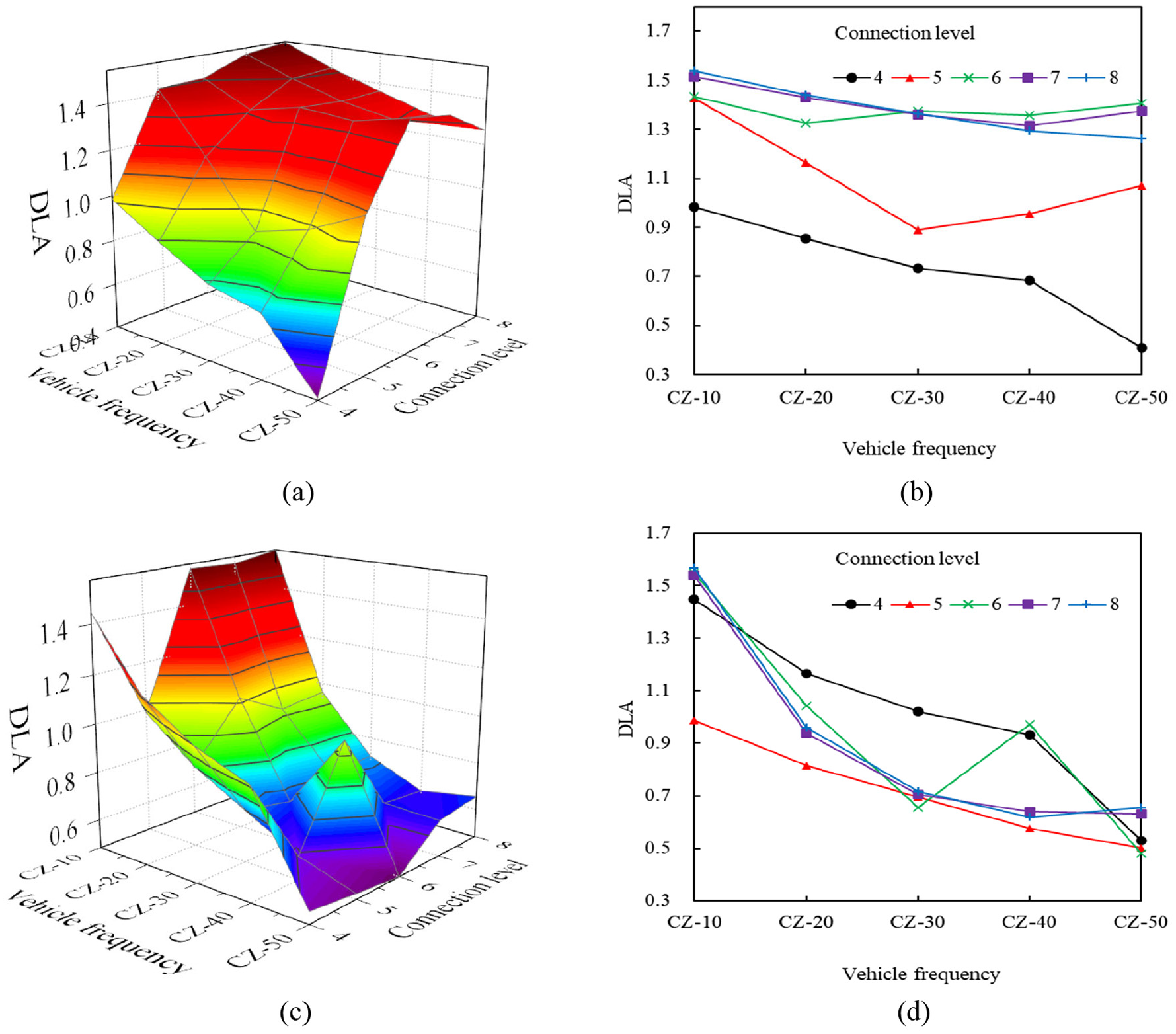
DLA value of the concrete slab and the steel girder under the influence of vehicle frequency: (a) the concrete slab (3D plot), (b) the concrete slab (2D plot), (c) the steel girder (3D plot), and (d) the steel girder (2D plot).

Figure 10 shows that the DLA of the concrete slab increases with increasing vehicle frequency and connection level. The DLA of the steel girder also increases with increasing vehicle frequency, but it first decreases and then increases as the connection level decreases. The dynamic effect of the steel-concrete composite beam bridge decreases when the shear connector stiffness decreases. When the shear stiffness reaches a critical value, the DLA is the lowest. Subsequently, the shear stiffness continues to decrease and the dynamic response increases sharply, which leads to the rapid destruction of the bridge.

Influence of vehicle speed

DLA value of the concrete slab and the steel girder under the influence of vehicle speed are shown in Figure 11.

Figure 11.

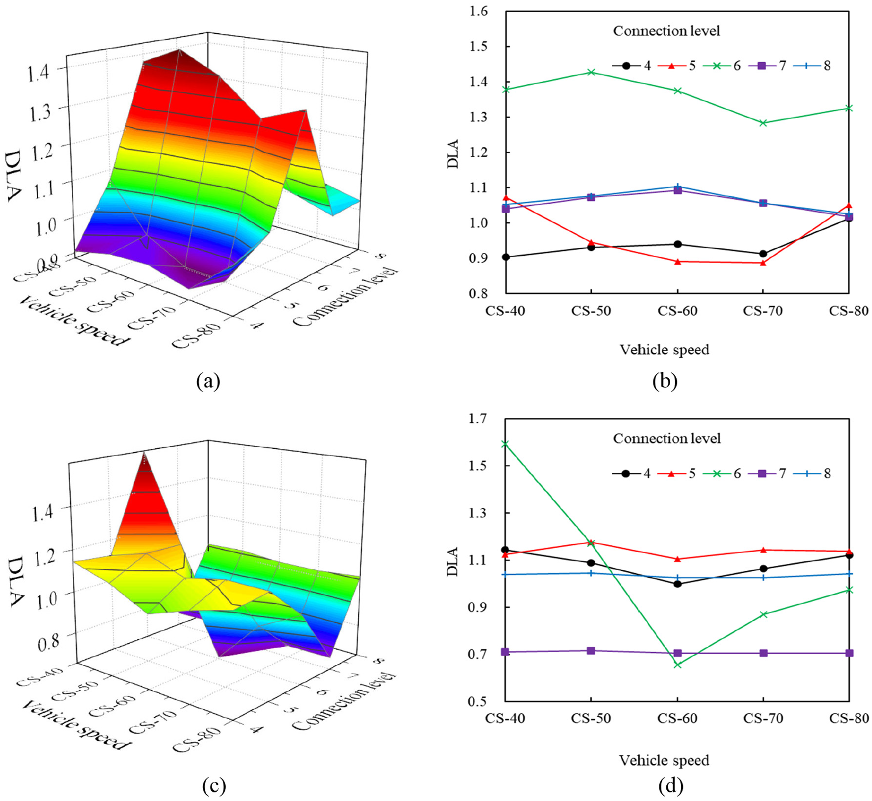
DLA value of the concrete slab and the steel girder under the influence of vehicle speed: (a) the concrete slab (3D plot), (b) the concrete slab (2D plot), (c) the steel girder (3D plot), and (d) the steel girder (2D plot).

Figure 11 shows that the DLA values of the concrete slab and steel beam are almost not affected by the vehicle speed at this point, but the DLA of the connection level is obvious. The DLA of the concrete slab gradually increases with increasing connection level and then decreases. The DLA of the steel beam first decreases and then increases. A trough appears when the connection level is 7.

The following results can be obtained from the above analysis. The DLA obtained from the stress of the concrete slab and steel beam is less affected by the vehicle speed and more affected by the connection level. The connection level trough also appears in other situations. Therefore, the bridge tends to be safe at the initial stage of the decrease in the shear connector stiffness, but the bridge safety decreases due to the influence of dynamic effects. After exceeding the critical shear stiffness, the bridge safety performance drops rapidly.

Influence of vehicle location

DLA value of the concrete slab and the steel girder under the influence of vehicle location are shown in Figure 12.

Figure 12.

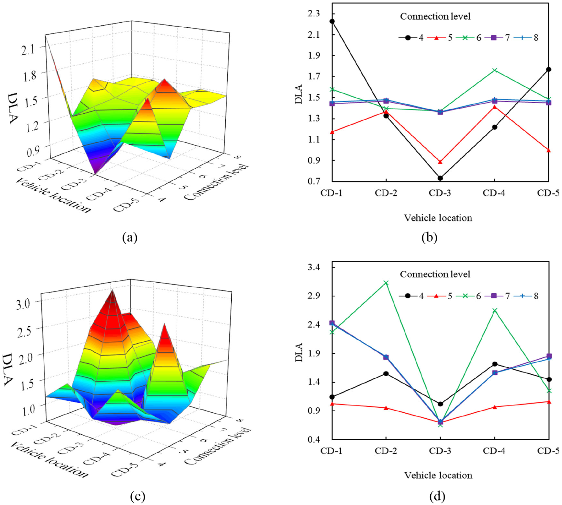
DLA value of the concrete slab and the steel girder under the influence of vehicle location: (a) the concrete slab (3D plot), (b) the concrete slab (2D plot), (c) the steel girder (3D plot), and (d) the steel girder (2D plot).

Figure 12 shows that when the vehicle is driving in the left and right lanes, the dynamic response of the bridge concrete slab and steel girder is relatively symmetric. In addition, the DLA is reduced to the lowest when the vehicle is driving on the central axis of the bridge. Bridges and vehicles are the safest under these conditions. The DLA of the concrete slabs and steel girder decreases and then increases with increasing connection level. A trough appears when the connection level is 5.

The conditions described above are more common in steel-concrete composite girder bridges. The composite girder bridge does not need to be over maintained. If the shear stiffness of the shear connectors is above the critical value, the bridge is regarded as safe. In addition, the vehicle is the safest when driven on the central axis, and the damage to the bridge is the lowest.

Influence of pavement roughness

DLA value of the concrete slab and the steel girder under the influence of pavement roughness are shown in Figure 13.

Figure 13.

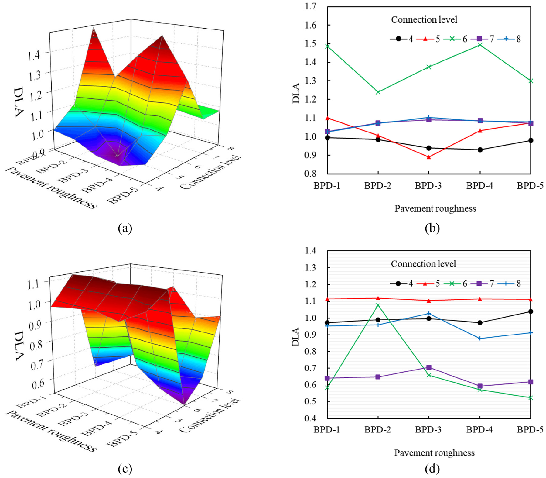
DLA value of the concrete slab and the steel girder under the influence of pavement roughness: (a) the concrete slab (3D plot), (b) the concrete slab (2D plot), (c) the steel girder (3D plot), and (d) the steel girder (2D plot).

Figure 13 shows that the DLA calculated by the stress of the concrete slab and the steel beam hardly changes with the pavement roughness. The DLA of the concrete slab increases and then decreases with increasing connection level. The DLA of the steel girder appears again in the conditions described above; that is, a trough appears when the connection level is 7.

The DLA calculated from the stress of the concrete slab and the steel girder is not sensitive to the changes in the pavement roughness. When the pavement roughness coefficient is low and the connection level is 6, the peak value of the DLA appears and is much larger than the others under the same connection level. The reason for this phenomenon is that the program does not converge when processing this parameter condition.

Dynamic responses of shearing studs

The dynamic response of interface connections is rarely studied by scholars. This paper studies the dynamic response of steel-concrete composite girder bridge shear connectors. Considering five connection levels, we focus on the DLA calculated from the longitudinal bridge deflection of the shear connector, the longitudinal bridge shear force and the vertical bridge axial force. Then, we use these three variables as the index to study the dynamic response of the interface connection.

Influence of bridge frequency

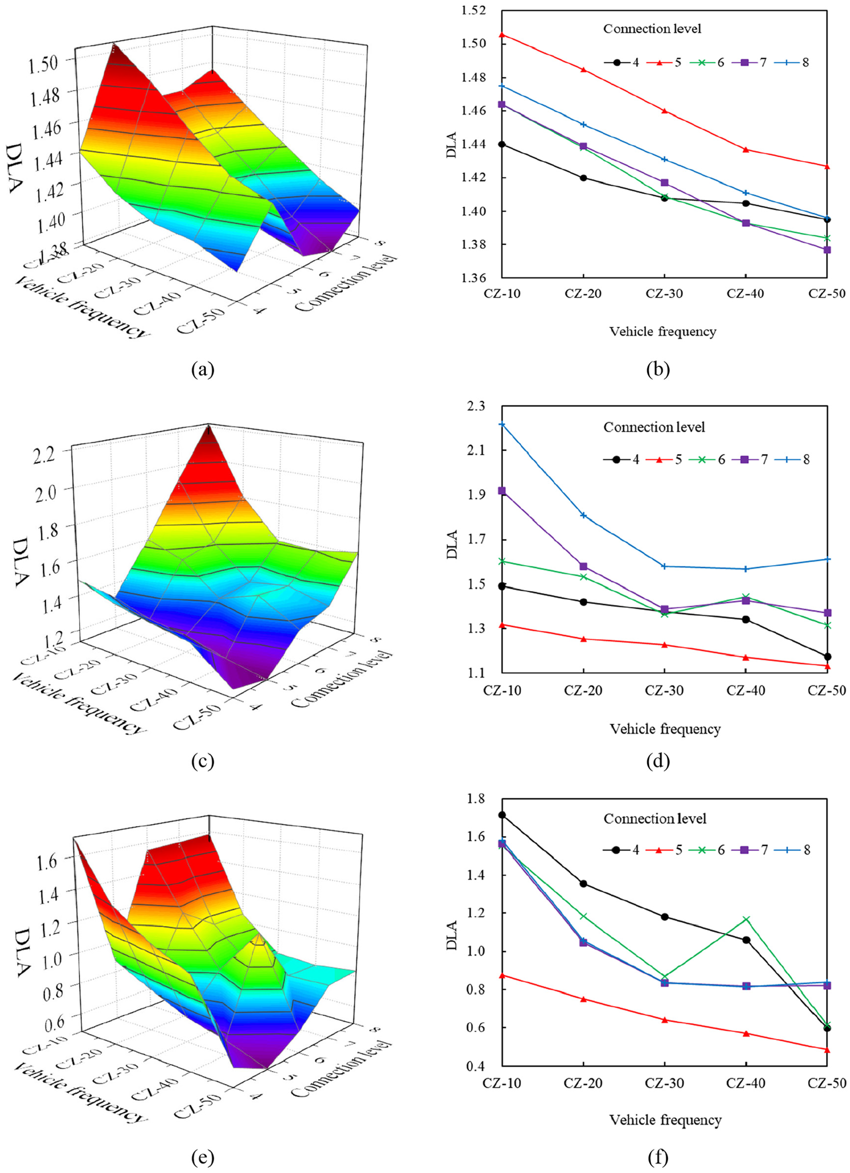
DLA value of the shear connector under the influence of bridge natural frequency are shown in Figure 14.

Figure 14.

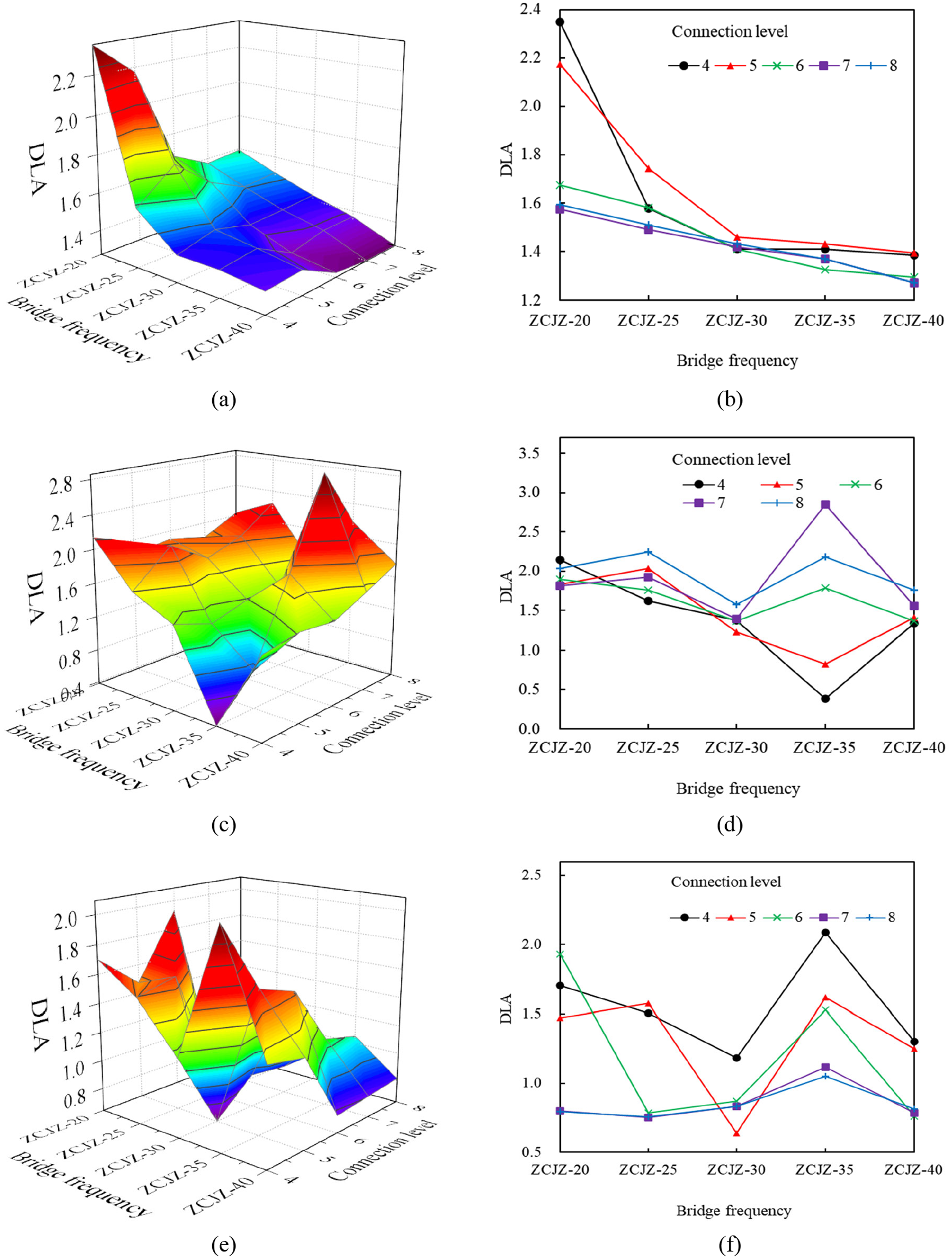
DLA value of the shear connector under the influence of bridge natural frequency: (a) the longitudinal deflection (3D plot), (b) the longitudinal deflection (2D plot), (c) the longitudinal shear force (3D plot), (d) the longitudinal shear force (2D plot), (e) the vertical axial force (3D plot), and (f) the vertical axial force (2D plot).

Figure 14 shows that the DLA of the longitudinal deflection of the shear connector decreases with increasing bridge span and connection level. The longitudinal deflection of the shear connector is the interface slip of the steel-concrete combination with the girder bridge. When the bridge mass becomes larger, the vehicle load decreases relative to the bridge weight, and the interface slip steadily decreases. The DLAs of the shear connector longitudinal shear force and the vertical axial force do not obviously change. The peak occurs when the bridge span is 35 m, and the DLAs change little at other locations. Therefore, it is best to limit steel-concrete composite girder bridges to a reasonable span during the design stage.

Influence of vehicle frequency

DLA value of the shear connector under the influence of vehicle frequency are shown in Figure 15.

Figure 15.

DLA value of the shear connector under the influence of vehicle frequency: (a) the longitudinal deflection (3D plot), (b) the longitudinal deflection (2D plot), (c) the longitudinal shear force (3D plot), (d) the longitudinal shear force (2D plot), (e) the vertical axial force (3D plot), and (f) the vertical axial force (2D plot).

Figure 15 shows that the changes in the DLA calculated by the longitudinal deflection, longitudinal shear and vertical axial force of the shear connector are relatively similar. That is, they all gradually increase with increasing vehicle frequency. The reason for this phenomenon is that the higher the vehicle frequency is, the more obvious the dynamic effect is. The DLA calculated by the longitudinal deflection and the longitudinal shear force does not change significantly with the connection level. The DLA calculated by the vertical axial force has a trough when the connection level is 5. It first decreases with increasing connection level and then gradually increases, gradually leveling off. The reason for the trend is similar to that above.

Influence of vehicle speed

DLA value of the shear connector under the influence of vehicle speed are shown in Figure 16.

Figure 16.

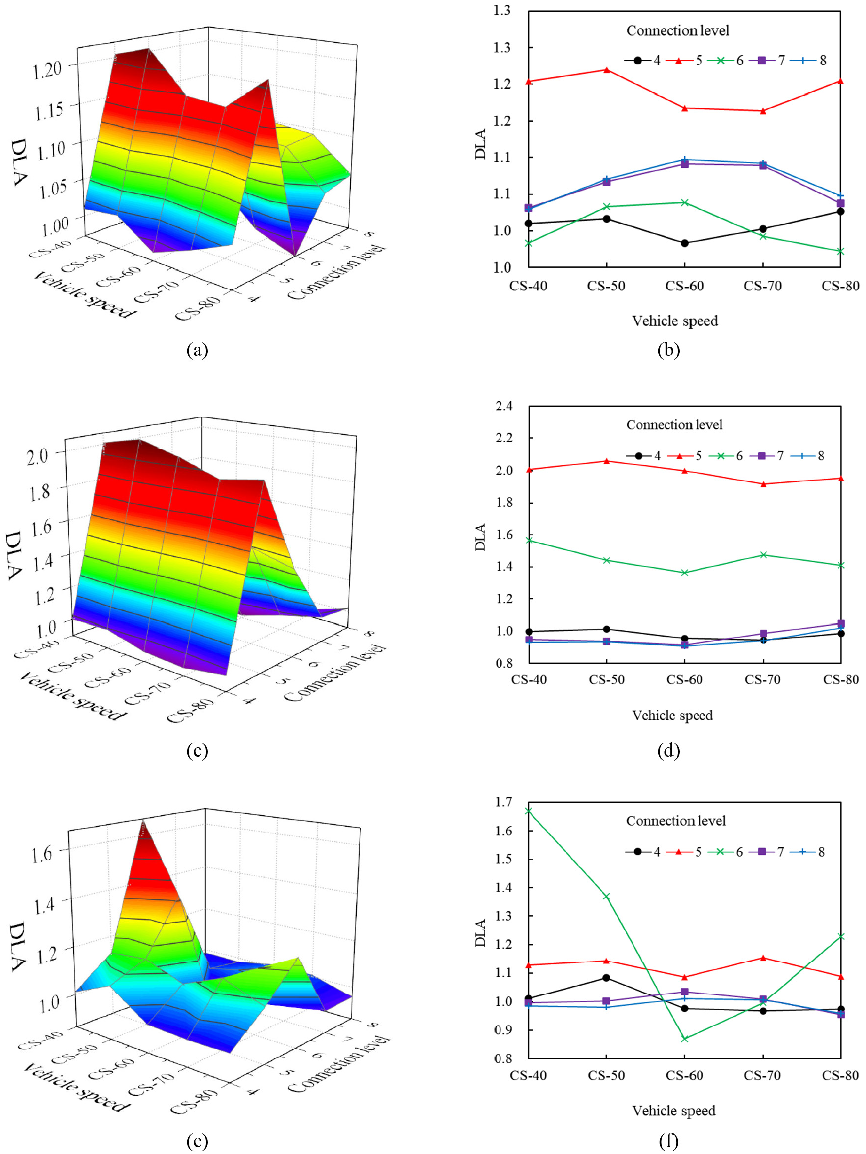
DLA value of the shear connector under the influence of vehicle speed: (a) the longitudinal deflection (3D plot), (b) the longitudinal deflection (2D plot), (c) the longitudinal shear force (3D plot), (d) the longitudinal shear force (2D plot), (e) the vertical axial force (3D plot), and (f) the vertical axial force (2D plot).

Figure 16 shows that the DLA calculated by the longitudinal deflection changes in a V-shaped curve with the speed change when the connection level is low. When the connection level is high, it changes in an N-shaped curve. The reason is that the influence of vehicle speed on the DLA generally changes in a W-shaped curve. Due to the different connection levels, the W-shaped curve falls on the peak and valley values, leading to two diametrically opposite forms of change.

In addition to the abovementioned law of changes, we analyze the following results. The DLA calculated by the longitudinal shear force shows an N-shaped curve change with the change in the connection level, and it hardly changes with the vehicle speed change. The DLA calculated by the vertical axial force has a small peak when the connection level is 5, and it is not sensitive to changes in vehicle speed. Rather, it only changes drastically when the connection level is 6 and almost does not change at the other connection levels.

Influence of vehicle location

DLA value of the shear connector under the influence of vehicle location are shown in Figure 17.

Figure 17.

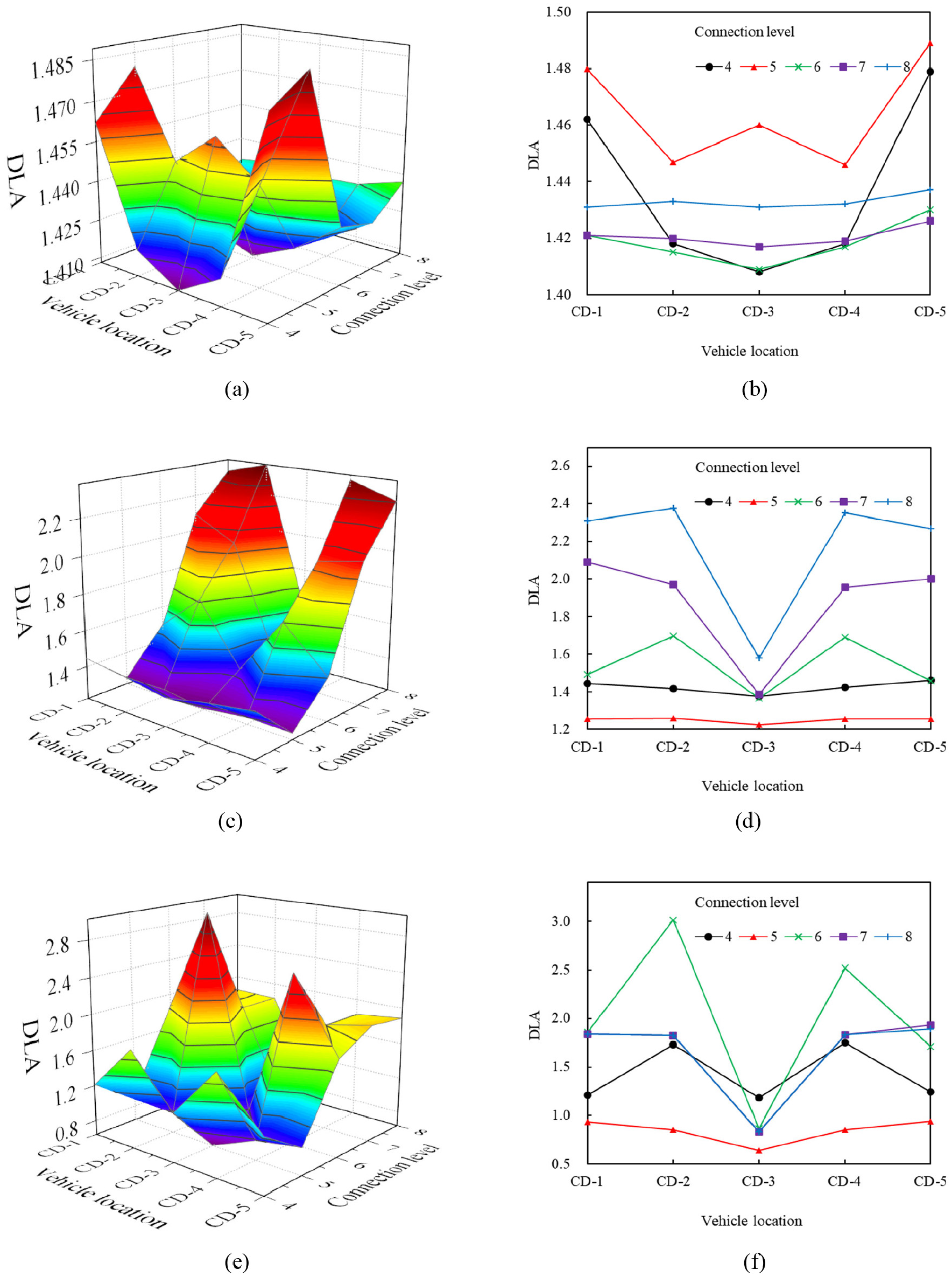
DLA value of the shear connector under the influence of vehicle location: (a) the longitudinal deflection (3D plot), (b) the longitudinal deflection (2D plot), (c) the longitudinal shear force (3D plot), (d) the longitudinal shear force (2D plot), (e) the vertical axial force (3D plot), and (f) the vertical axial force (2D plot).

Figure 17 shows that the DLA value of the shear connector changes with the connection level change and the position of the vehicle center axis. This change presents an axisymmetric condition; that is, the DLA of the vehicle when driving on the left and on the right is similar, and the DLA at a lower connection level and at a higher connection level is similar. When the connection level is 5, it is safest to drive on the central bridge axis.

Influence of pavement roughness

DLA value of the shear connector under the influence of pavement roughness are shown in Figure 18.

Figure 18.

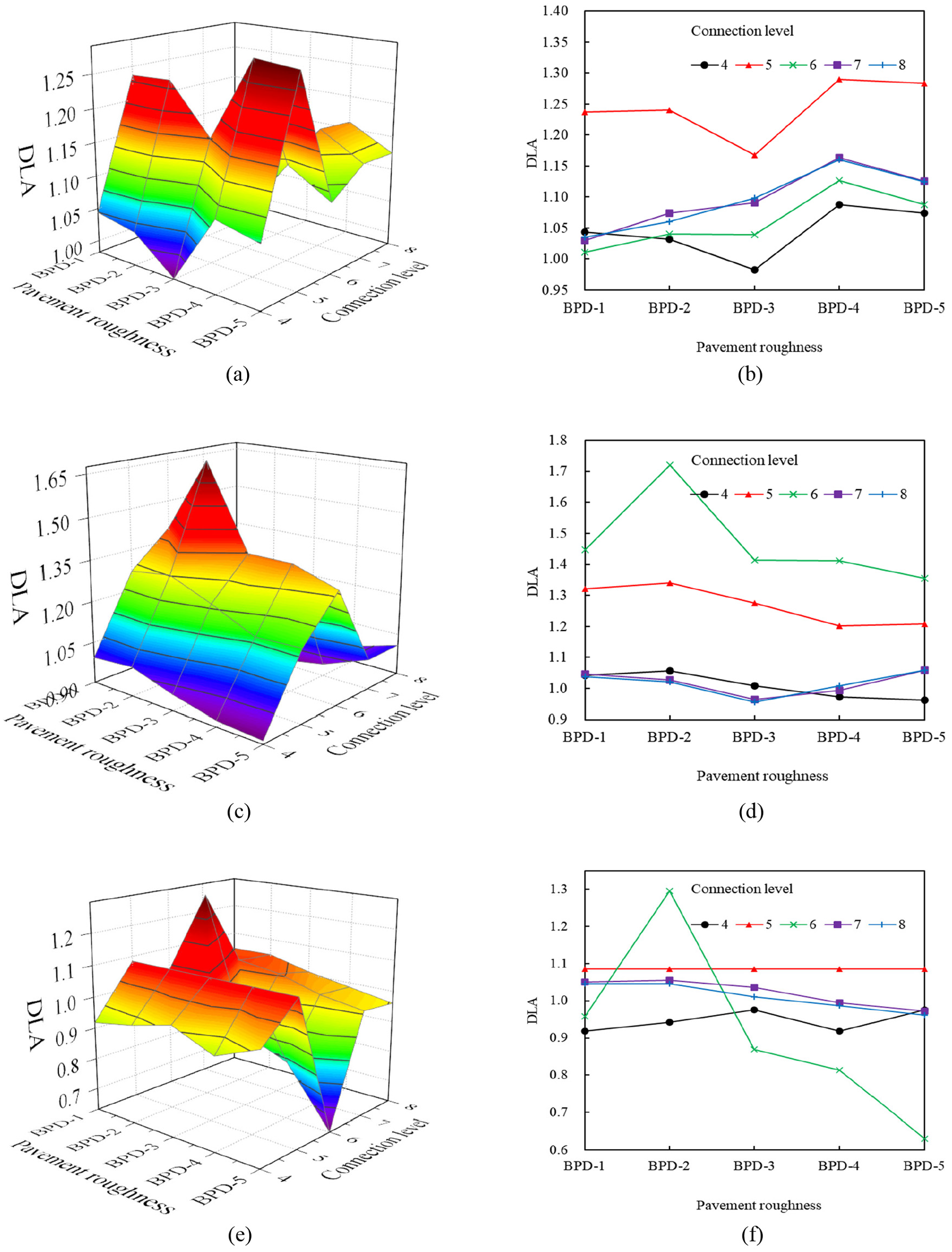
DLA value of the shear connector under the influence of pavement roughness: (a) the longitudinal deflection (3D plot), (b) the longitudinal deflection (2D plot), (c) the longitudinal shear force (3D plot), (d) the longitudinal shear force (2D plot), (e) the vertical axial force (3D plot), and (f) the vertical axial force (2D plot).

Figure 18 shows that the DLA calculated by the longitudinal deflection exhibits a W-shaped curve change with the change in the connection level. The DLA calculated by the longitudinal shear force has a peak when the connection level is 6, and the DLA calculated by the vertical axial force has a low when the connection level is 6. The DLA almost does not change with the pavement roughness under other connection levels.

In general, the DLA change of the shear connector under the influence of the pavement roughness is similar to that under the influence of the vehicle speed. The DLA calculated from the longitudinal deflection, longitudinal shear and vertical axial force have different trends. When the pavement level is good and the connection level is 6, the DLA reaches the maximum.

Conclusion

This paper establishes a simply supported steel-concrete composite girder bridge model and an entire vehicle model. The model considers the influence of the pavement roughness and vehicle-bridge coupled vibration and establishes five connection levels. Based on the numerical simulation, the conclusions of the influence of bridge natural frequency, vehicle frequency, vehicle speed, vehicle position and pavement roughness on the DLA of the composite beam bridge are as follows:

Changes in bridge frequency and vehicle frequency can produce significant changes in the DLA. The closer frequencies of the two are, the more significant DLAs increase, and the more likely it is to cause resonance.

The impact of vehicle speed on the DLA is generally W-shaped. Since different connection levels correspond to different peaks and valleys of the W-shaped curve, when the DLA is low and high, the DLA changes with the vehicle speed in the V-shaped and N-shaped curves, respectively.

The change in the DLA of the vehicle lateral position is highly symmetrical, and the DLA value at the side beam is larger than that of the center beam. This result is consistent with the trends from simply supported beams and conforms to common sense. In dangerous sections, we should try to drive in the middle of the bridge to ensure that people and the bridge will be safer.

DLAs of different pavement roughnesses have different regularities. For the DLA calculated by deflection, the DLA increases with increasing pavement roughness coefficients. The DLA calculated by stress is barely affected by the pavement roughness. For the DLA of the shear connector, its change with the pavement roughness is similar to that of the vehicle speed.

Footnotes

Declaration of conflicting interests

The author(s) declared no potential conflicts of interest with respect to the research, authorship, and/or publication of this article.

Funding

The author(s) disclosed receipt of the following financial support for the research, authorship, and/or publication of this article: This work was supported by the National Natural Science Foundation of China (51778194), the China Postdoctoral Science Foundation (2017M621282), and the Fundamental Research Funds for the Central Universities (HIT. NSRIF. 2019056).

ORCID iD

Qingfei Gao

References

Nie

Wang

Gou

, et al. Technological development and engineering applications of novel steel-concrete composite structures. Front Struct Civ Eng 2019; 13(1): 1–14.

Nie

Tao

, et al. Advances of research on steel-concrete composite bridges. China Civ Eng J 2012; 45(6): 110–122.

Xue

Liu

, et al. Static behavior of multi-stud shear connectors for steel-concrete composite bridge. J Constr Steel Res 2012; 74: 1–7.

Xiao

Behavior of perforated shear connectors in steel–concrete composite joints of hybrid bridges. J Bridge Eng 2017; 22(4): 04016135.

Lee

Shim

Chang

SP.

Static and fatigue behavior of large stud shear connectors for steel–concrete composite bridges. J Constr Steel Res 2005; 61(9): 1270–1285.

Khorramian

Maleki

Shariati

, et al. Numerical analysis of tilted angle shear connectors in steel-concrete composite systems. Steel Compos Struct 2017; 23(1): 67–85.

Gao

Dong

Cui

, et al. Fatigue performance of profiled steel sheeting–concrete bridge decks subjected to vehicular loads. Eng Struct 2020; 213: 110558.

Xue

Study on steel-concrete composite beams under low-reversed cyclic loading. Earthq Eng Eng Vib 2002; 22(6): 65–70.

Jia

Lan

Zheng

, et al. Assessment on required separation length between adjacent bridge segments to avoid pounding. Soil Dyn Earthq Eng 2019; 120: 398–407.

10.

Jia

Zhao

, et al. Probabilistic pounding analysis of high-pier continuous rigid frame bridge with actual site condition. Earthq Struct 2018; 15(2): 193–202.

11.

Zhang

Liu

Damage detection of bridges monitored within one cluster based on the residual between the cumulative distribution functions of strain monitoring data. Struct Health Monit 2020; 19(6): 1–26.

12.

Nie

Cai

CS.

Steel-concrete composite beams considering shear slip effects. J Struct Eng 2003; 129(4): 495–506.

13.

Ranzi

Zona

A steel–concrete composite beam model with partial interaction including the shear deformability of the steel component. Eng Struct 2007; 29(11): 3026–3041.

14.

Liang

Bradford

, et al. Strength analysis of steel–concrete composite beams in combined bending and shear. J Struct Eng 2005; 131(10): 1593–1600.

15.

Jiang

Feng

Zhou

, et al. Analysis on natural vibration characteristics of steel-concrete composite truss beam. Steel Compos Struct 2018; 26(1): 79–87.

16.

Hou

Xia

Wang

, et al. Dynamic analysis and model test on steel-concrete composite beams under moving loads. Steel Compos Struct 2015; 18(3): 565–582.

17.

Tahmasebinia

Ranzi

Zona

. Beam tests of composite steel-concrete members: a three-dimensional finite element model. Int J Steel Struct 201; 12(1): 37–45.

18.

Wang

Huang

Liu

, et al. Experimental investigation of steel-concrete composite beams with different degrees of shear connection under monotonic and fatigue loads. Adv Struct Eng 2018; 21(2): 227–240.

19.

Zhang

Liu

Zhang

, et al. Time interval of multiple crossings of the Wiener process and a fixed threshold in engineering. Mech Syst Signal Process 2020; 135: 106389.

20.

Han

Yuan

Vibration of vehicle-bridge coupling system with measured correlated road surface roughness. Struct Eng Mech 2014; 51(2): 315–331.

21.

Liu

Zhang

, et al. Applying constrained layer damping to reduce vibration and noise from a steel-concrete composite bridge: an experimental and numerical investigation. J Sandw Struct Mater 2020; 22(6): 1743–1769.

22.

Szurgott

Bernacki

Modelling of steel-concrete bridges subjected to a moving high-speed train. Int J Simul Model 2020; 19(1): 29–40.

23.

Matsuoka

Collina

Somaschini

, et al. Influence of local deck vibrations on the evaluation of the maximum acceleration of a steel-concrete composite bridge for a high-speed railway. Eng Struct 2019; 200: 109736.

24.

Wang

Zhu

Dynamic response analysis of monorail steel-concrete composite beam-train interaction system considering slip effect. Eng Struct 2018; 160: 257–269.

25.

Madrazo-Aguirre

Ruiz-Teran

Wadee

MA.

Dynamic behaviour of steel–concrete composite under-deck cable-stayed bridges under the action of moving loads. Eng Struct 2015; 103: 260–274.

26.

Kwon

Lee

Moon

, et al. Dynamic interaction analysis of urban transit maglev vehicle and guideway suspension bridge subjected to gusty wind. Eng Struct 2008; 30(12): 3445–3456.

27.

Cai

Zhu

, et al. Dynamic interaction of suspension-type monorail vehicle and bridge: numerical simulation and experiment. Mech Syst Signal Process 2019; 118: 388–407.

28.

Gao

Cui

, et al. Optimal layout of sensors in large-span cable-stayed bridges subjected to moving vehicular loads. Int J Distrib Sens Netw 2020; 16(1): 155014771 9899376.

29.

Wang

Yan

Deng

, et al. Dynamic analysis of a cable-stayed concrete-filled steel tube arch bridge under vehicle loading. J Bridge Eng 2015; 20(5): 04014082.

30.

Kong

Cai

, et al. New strategy of substructure method to model long-span hybrid cable-stayed bridges under vehicle-induced vibration. Eng Struct 2012; 34: 421–435.

31.

Chen

Cai

CS.

Equivalent wheel load approach for slender cable-stayed bridge fatigue assessment under traffic and wind: feasibility study. J Bridge Eng 2007; 12(6): 755–764.

32.

Chen

Huang

YF.

Coupling vibration of vehicle-bridge system. Appl Math Mech 2004; 25(4): 390–395.

33.

Deng

, et al. Research progress in theory and applications of highway vehicle-bridge coupling vibration. China J Highw Transp 2018; 31(7): 38–54.

34.

Zhang

State-of-the-art review and trend of studies on coupling vibration for vehicle and highway bridge system. Eng Mech 2008; 3: 230–240.

Numerical investigation of the dynamic responses of steel-concrete girder bridges subjected to moving vehicular loads

Abstract

Keywords

Introduction

Vehicle-bridge coupled vibration

Numerical simulation

Sample selection of the steel-concrete composite simply supported girder bridge

Moving vehicle load parameters

Simulation of pavement roughness

Classification of interface connection levels between steel girder and concrete slab

Dynamic responses of concrete slabs

Influence of bridge frequency

Influence of vehicle frequency

Influence of vehicle speed

Influence of vehicle location

Influence of pavement roughness

Dynamic responses of steel girders

Influence of bridge frequency

Influence of vehicle frequency

Influence of vehicle speed

Influence of vehicle location

Influence of pavement roughness

Dynamic responses of shearing studs

Influence of bridge frequency

Influence of vehicle frequency

Influence of vehicle speed

Influence of vehicle location

Influence of pavement roughness

Conclusion

Footnotes

Declaration of conflicting interests

Funding

ORCID iD

References