
Abstract
As macroscopic rough terrains are time varying and full of local topographic mutations, stable locomotions of legged robots moving through such terrains in a fixed gait form can be hardly obtained. This problem becomes more severe as the size and weight of the robot increase. An ideal pre-planned gait changing method can also be hardly designed due to the same limitations. Aiming to solve the problem, a new kind of free gait controller applied to a large-scale hexapod robot with heavy load is developed. The controller consists of two parts, a free gait planner and a gait regulator. Based on the observed macro terrain changes, the free gait planner adopts the macro terrain recognition method and the status searching method for selecting the best leg support status automatically. The gait regulator is adopted for the correction of the selected status to cope with local topographic mutations. Detailed simulation experiments are presented to demonstrate that, with the designed controller, the adopted hexapod robot can change moving gaits automatically in terms of the terrain conditions and obtain stable locomotions through rough terrains.
Keywords
Introduction
Compared with wheeled robots, bionic legged robots achieve better motion performances using discontinuous ground support.1–3 For the goal of large load field transportations, legged robots in large size and weight are developed. However, a good solution is needed to deal with the problem of improving the walking stability and environmental adaptability of large-scale legged robots under harsh external environments, 4 because with the increases of a robot’s size and mass, the ever-larger contact impact between the robot’s feet and the ground will significantly affect the walking attitude of the robot. Attitude recovery is tough for a large-scale robot with a heavy load because of the great inertia of the robot body. Besides, compared with small robots, once instability occurs, the robot with large size and mass will be hard to recover simply by the manipulator alone. This may also cause irreversible damage to the mechanical components. Therefore, how to improve the moving stability of large robots arouses the interests of scholars and controllers based on different methods for achieving stable motions have been developed.5–7 Among all kinds of controllers, the walking mode controller is one of the most basic and important controllers.
The walking mode of legged robots is mainly manifested as gait. Usually, the walking motion of a legged robot mainly adopts a fixed gait, because this will simplify the control system, especially when the robot is small and lightweight. A legged robot walking with a fixed gait form can achieve good stability on a uniform terrain, but when the external terrain becomes rough, the situation will be different. The unfixed gait named as free gait can be a good way to solve this problem. The ability to change moving states in terms of changes in the external environment can be ensured if a free gait controller is applied to the robot. Therefore, better stability and adaptability can be achieved.
The concept of free gait was first proposed by McGhee and Iswandhi. 8 In their control scheme, the step sequence was generated by the continuous computation of the static stability evaluation norm. Limited by the low computational efficiency, the engineering application was not good at that time. Based on the optimization of energy consumption, Hirose 9 designed an adaptive gait control method for a quadruped robot. Bai et al. 10 introduced a gait form called primary/secondary gait to control the robot motions in common and obstacle negotiation situations. In these controllers, kinematic constraints are not taken into account and this may cause “locking up” between the legs due to the overrun of the motion range. To solve this problem, Pal and Jayarajan 11 proposed a free gait controller for hexapod walking based on the graph searching method. The kinematic constraints were taken into account to avoid this situation. Similar control methods can be found in the study by Chen et al. 12 and the study by Pack and Kang. 13 Based on a vision sensor and laser sensors, topographic information was obtained and introduced into a free gait controller developed by Belter. 14 In this controller, A* and RRT-Connect algorithms were used. Globally optimal solutions of the gait form and the motion path could be obtained. Effectiveness verifications of moving through rough terrains were carried out on a hexapod robot. In fact, these free gait controllers are almost all based on optimization methods under different user-defined constraints. Many other kinds of controllers based on optimization methods can be found in the studies of walking mode designing.15–19
In addition to the controllers based on optimization methods, bionic controllers are also widely studied, which can be mainly divided into controllers based on central pattern generators (CPGs) and walking rules. Since Shik et al. 20 announced that rhythmic motions of some animals and insects were generated by CPGs, many studies of applying the CPG control principles to real legged robots have been carried out.21–24 Kirchner et al. 25 established a CPG model to integrate the control and feedback signals. Through this model, adaptive motions of the robot SCORPION through unknown environments were generated. Another similar controller was also developed by them and applied to the hexapod robot called SCARABAEUS. 26 Kimura et al. 27 established a control scheme based on a CPG model for the robot Tekken and verified the effectiveness of the controller through obstacle negotiation motions. Espinal et al. 28 developed a CPG-based controller to generate hexapod locomotion of their robot automatically, and a heuristic algorithm was adopted to obtain the parameters of their CPG model. Gay et al. 29 presented a control scheme based on CPG principles to achieve stable locomotions and balance control of a quadruped robot. In this control scheme, a neural network was adopted to represent sensory feedbacks inside the CPG dynamics. The weights of the net were optimized using the particle swarm optimization algorithm. Compared with an open-loop control scheme, significant walking improvements of the robot were obtained.
Based on the studies of stick insects, Cruse et al. 30 revealed six rules of hexapod walking and designed a simple neural network called walknet to realize hexapod walking motions. During walking, gait parameters were generated by walknet according to the motion states of the robot. Inspired by Cruse’s rules, many free gait controllers have been developed by scholars.31,32 Goerner and Hirzinger 33 designed a gait controller for the robot DLR-Crawler based on Cruse’s rules. Sensory feedback signals of foot forces were introduced into the controllers to regulate the parameters of the walking rules. Stable rough terrain walking of the robot was achieved. Estremera and De Santos 34 designed a rule-based free gait controller for the robot SILO4 to move across the irregular terrain. Stability margin was taken into account to regulate the motion of the robot. Similar idea was also adopted by Johnson, and Sahin 35 to design their controllers for hexapod walking.
From the current research achievements of the free gait controllers, it can be found that although the free gait controllers based on the optimization methods can improve the motion performances of legged robots in some specific aspects, they also have limitations like long optimization time and falling into the local optimal solutions. In addition, it is usually necessary to know the external environment information in advance. Free gait controllers based on CPGs usually do not need to know the exact models of the environments in advance, but the complexity of computation cannot be ignored. Free gait controllers based on walking rules seem to be the simplest controllers. But walking rules cannot be adopted alone without other optimization algorithms if appropriate parameters of the controller are needed. Furthermore, the computational efficiency may not be good.
In summary, the performance of a multifunctional free gait controller should not be limited by the external environment. Meanwhile, its structure should be simple. Considering the characteristics and requirements of heavy robots, a free gait controller designed for a heavy load hexapod robot is proposed in this article. Compared with other free gait controllers, the proposed free gait controller is simple and multifunctional. Without any complex nonlinear computation, the designed controller is fit for real-time control systems. Besides, applications of the controller are not limited by different structures of hexapod robots. Adaptive motion demands in unknown environments can also be realized without any advanced sensors like vision sensors or laser sensors.
This article is organized as follows: in the second part, a brief overview of the heavy load hexapod robot and the controller structure are introduced. In the third part, the free gait controller which consists of a free gait planner and a gait regulator is introduced in detail. In the fourth part, the effectiveness of the free gait controller is validated through several comparative simulation experiments.
System overview
The heavy load hexapod robot
A heavy load hexapod robot is employed to validate the effectiveness of the proposed free gait controller because of two reasons: first, the six-legged structure determines that the robot has a variety of leg motion combinations, namely, the robot has multiple walking gaits; second, because of the heavy load feature, small terrain changes will cause a great impact on the walking stability of the robot. When the external terrain becomes more complex, this effect may be magnified exponentially. Therefore, the heavy load robot has a higher demand for walking stability than the lightweight robots. Structure of the heavy load hexapod robot is shown in Figure 1(a) and the schematic leg structure of the robot is shown in Figure 1(b). The overall mass of the robot is 5 tons. The left legs are named as leg 1, leg 2, and leg 3, respectively. The right legs are named as leg 4, leg 5, and leg 6, respectively. The leg structure of the robot is a parallelogram pantograph mechanism. Three joints are assembled on the leg to drive the movement of the leg. The vertical joint controls the leg’s vertical movement, the horizontal joint controls the leg’s horizontal movement, and the sway joint controls the leg’s sway movement, as shown in Figure 1(b).

The heavy load hexapod robot structure: (a) robot structure and (b) leg structure.
The walking motion of the robot legs is divided into a support status and a swing status, similar to other legged robots. During the support status, the support legs contact the ground and push the robot body forward. During the swing status, the swing legs remain swinging forward to reach the planned foot landing positions. At the end of the swing status, the swinging legs convert into the support legs. At the end of the support status, some of the support legs convert into swing legs in terms of the selected gait form. Force sensors are assembled on each foot to detect if a leg is in the support status. An inertial navigation element is assembled on the robot body to detect and record the body postures.
Brief structure of the controller
The schematic diagram of the free gait controller is shown in Figure 2.

Schematic diagram of the free gait controller.
The free gait controller mainly consists of a free gait planner and a gait regulator. The free gait planner and the gait regulator are complementary. During a hexapod walking, sensory feedback signals of the foot positions are employed into the free gait planner and the gait regulator. The slope angle of the terrain is first observed through a macro terrain recognition method. Based on the slope angle, alternative support statuses (namely, the alternative gait forms) can be determined from multiple gaits. Stability constraint and kinematic constraint are both taken into account in the free gait planner. Based on the continuous computations of the alternative gait stabilities and kinematic margins, the alternative gaits can be further sifted and a target gait can be selected. The free gait planner is commonly used to deal with regular slope climbing issues. When the robot comes across irregular terrains with obstacles or ditches, sensory foot force signals will be employed into the gait regular. Based on the judgment of the robot motion state, the gait regulator starts to make corrections of both the target gait form and the conventional foot trajectories generated by the trajectory generator of the robot. Through the cooperative working of the gait planner and the gait regulator, the free gait controller can work in a loop-locked way and avoid problems of the conventional open-loop control schemes. The detailed designs of the controller will be introduced in the third part of the article.
Free gait controller
Free gait planner
Stable support statuses for the hexapod robot
For a legged robot, each leg has two motion statuses, namely, the swing status and the support status. Therefore, a hexapod robot has 26 = 64 possible walking states. However, most of them are unstable or critically stable. In order to realize stable walking motions, 18 stable support statuses that could be applied to gait transitions were established, as shown in Table 1.
Stable support statuses.

In Table 1, black dots indicate the support legs, whereas 1 and 0 indicate the support status and the swing status, respectively.
The former 17 statuses can be divided into three groups, namely, the three-legged support status, the four-legged support status, and the five-legged support status. Neglecting the changes of local topography, the change of macro terrain mainly refers to the slope angle. The number of support legs should be selected in terms of different slope angles because when the slope angle increases, the increased number of support legs will improve the walking stability of the robot. In order to achieve this goal, the relationship between the number of support legs and the slope angle was established, as shown in Table 2.
Relationship between support statuses and slope angle.
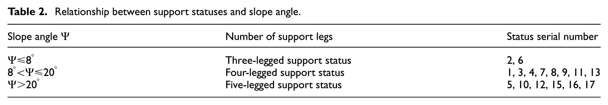
Although the support status can be selected according to Table 2, the slope angle always changes with time and is difficult to know in advance. In addition, even if the slope angle is determined, a plurality of support statuses can be selected. Therefore, to allow the robot to determine the optimal support status automatically, a macroscopic terrain recognition method was designed. Some constraints were also employed to enable the robot to search and select the optimal support status from Table 2.
The macro terrain recognition method
Usually, it is difficult to know the exact terrain conditions without a vision sensor or laser sensors. However, if only the tilt angle is needed to be identified without a very high precision, things will become easier. As described in the second part of the article, foot force sensors are assembled on the robot feet. On this basis, a macro terrain recognition method was established.
The nonzero vertical value of a foot force sensor indicates that the leg is in support status. Based on this, all support legs can be detected. In other words, the support status of the robot can be determined. Coordinate systems were set up, as shown in Figure 3.

Coordinate systems for the hexapod robot.
In Figure 3,
For any foot in the support status, the sensory values of each joint position are recorded. The positions of the robot’s supporting feet in the body coordinate system, namely,

where

Vector
The three Euler angles

where
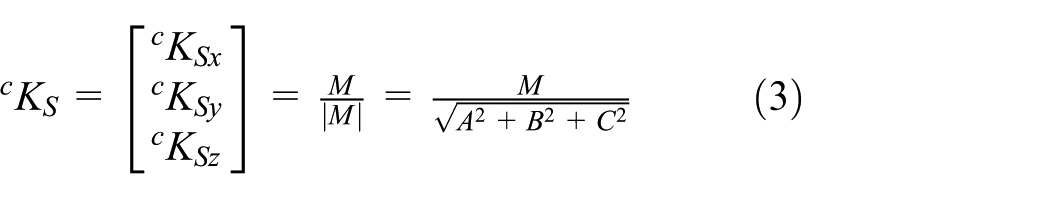
Based on the normal vector of the global coordinate system

In terms of the observed slope angle
Motion constraints for choosing support status
Based on the identified slope angle, the robot can choose the number of support legs as shown in Table 2. But corresponding to one slope angle, there are still more than one statuses which can be selected. In order to make the robot choose the best support status, two motion constraints were taken into account.
The first one is the stability constraint. The static stability margin, namely, the minimum distance from the projection of the center of gravity along the direction of gravity on the supporting plane to each edge of the support polygon, was selected to evaluate the stability of the robot. In order to show the static stability margin more intuitively, a hexapod robot in five-legged support status is taken as an example as shown in Figure 4.
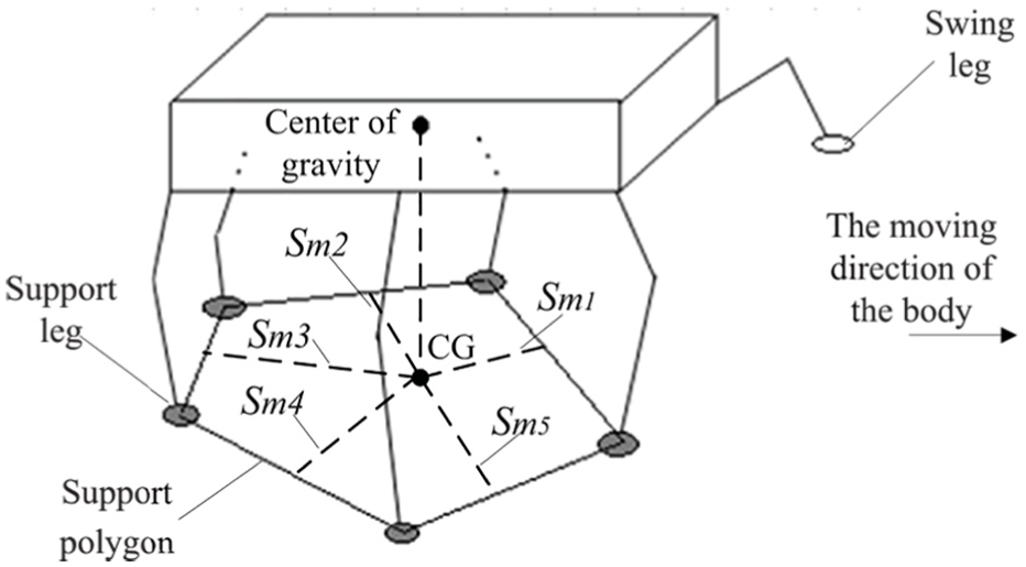
Static stability margin of a hexapod robot.
In Figure 4,
Based on the static stability margin, a stability constraint was established, namely, the robot must choose the target support status which has the largest change in the stability margins from the current support status to all the alternative target support statuses. The change in stability margins can be written as shown in equation (6)

where
The second constraint is the kinematic constraint. For a legged robot, the forward motion of the robot body is pushed by the support legs. Each support leg has a rear extreme position (PEP) which is limited by the mechanical structure of the robot. If an improper support status is selected, the support legs may move out of their motion ranges and the robot may lose its stability. In order to avoid this situation, kinematic constraint was taken into account. The kinematic margin of one leg, namely, the distance between the current position of the support foot and its PEP, can be adopted to define the kinematic range, as shown in Figure 5.
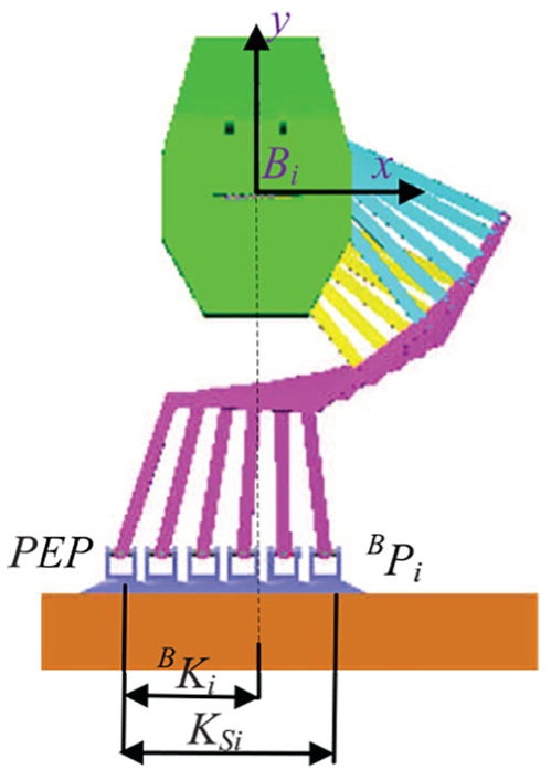
Kinematic margin of a support leg.
In Figure 5,

Based on the kinematic margin of one leg, the kinematic constraint was established. Similar to the stability constraint, the change in the kinematic margin of all the support legs from the current support status to all the alternative support statuses was adopted to judge the kinematic performance of the robot, as shown in equation (8)

where
It is important to note that, for leg

where

Based on the proposed constraints, namely, equations (6) and (8), an evaluation function was established, as shown in equation (11)

The evaluation function
Gait regulator
The gait regulator is adopted for correcting the target support status to deal with local topographic mutations. For instance, when one swing leg hits an obstacle and cannot continue swinging as planned, or, because of the presence of the ditches on the terrain, the planned landing position of one swinging leg is not detected, the moving state of the robot will be hampered. In order to solve this problem, a gait regulator was established.
Switch rules for motion status transition
During an ideal motion, swing legs of a hexapod robot touch the ground simultaneously as planned. But, on the contrary, the landing time of any swing leg may be earlier or delayed due to the mutations on the rugged terrain. When a swing leg touches the ground in advance, the swing status should be ended to avoid lifting the robot body. When the swing status of one leg is delayed, the swing status should be kept and the support statuses of other legs should be kept to avoid losing stability suddenly. To solve this problem, two more moving statuses called “swing-kept status” and “support-kept status” were introduced into the gait regulator.
The two new statuses may obstruct the planned moving status of the robot and control logical conflicts may occur. To avoid this situation, four switch rules for the moving status transition were established as follows:
The robot must be able to switch the movements of all legs in time according to the sudden change of the terrain;
When any swing leg is in the swing-kept status, all other legs must be in support statuses;
When the motion status of any leg changes, the moving velocity of the leg must be successive to avoid losing stability of the robot which is caused by the velocity mutation;
When all swing legs touch the ground, the robot continues to choose the best moving status using the free gait planner.
The leg motion adjustment method for ditch negotiation
Topographic mutations can be divided into two main types: obstacles (such as big rocks or fences) and ditches. The gait regulator is mainly designed for coping with these two types of terrain mutations. Inspired by biological reflection, an obstacle negotiation method for the hexapod robot adopted has already been established and verified in the authors’ earlier work. 36 In this article, a leg motion adjustment method for ditch negotiation was established.
Usually, when the vertical foot force of one leg is detected larger than the set value (the set value is usually zero), the leg begins to convert into the support status at the end of the swing status. Nevertheless, when there is a ditch on the local surface and the swing leg moves into the ditch at the end of the swing status, the vertical foot force of the leg will still be zero. At this time, if the robot is still moving forward, it will make a “misstep” and become unstable. Therefore, the motion status should be adjusted.
To deal with this problem, the swing leg which does not touch the ground as planned should keep swinging, namely, it should be in the swing-kept status. Then the leg finds a new foot landing position through continuously searching forward. When the vertical foot force of this leg is detected larger than the set value, it can convert into support status. According to the second switch rule, when the swing leg is in the swing-kept status, the other support legs should delay the status switching time and convert into support-kept statuses. The robot can return to its original moving status until a new foot landing position is detected. The whole process is shown in Figure 6.

Ditch negotiation process.
In Figure 6,
The searching process of the swing leg can be divided into three circumstances, as shown in Figure 7.

New foot landing position searching process: (a) downward searching process, (b)multiple searching process and (c) failed searching and returning process.
In Figure 7(a), a new foot landing position is detected directly through downward movement of the leg. In Figure 7(b), a new foot landing position is detected through multiple searching movements of the leg. In Figure 7(c), when the swing leg moves to its maximum range of motion, a new foot landing position cannot still be detected through multiple searching movements. Then this leg should return to the original position. At this moment, the ditch is too wide for the robot to pass. The robot should find another way to pass it.
During the searching process, the swing trajectory should be redesigned. In terms of the situation shown in Figure 7(a), the swing trajectory of the leg along the

where

where
Corresponding to the situation shown in Figure 7(b), the swing trajectory of the leg along the
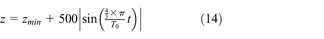
where
If a new foot landing position is still not detected through multiple searching movements, the swing leg should return to its original position, just as the situation shown in Figure 7(c). The backward swing trajectory of the leg is designed based on Bézier spline. The Bézier spline adopted here has the same form as in the authors’ previous work.
36
The sketch of the backward swing trajectory is shown in Figure 8, where AEP indicates the foot position when the searching leg moves to its maximum range of motion and

Backward swing trajectory of the searching leg.
Simulation results
Simulation experiments were carried out on the ADAMS-Simulink co-simulation platform to verify the effectiveness of the controller. First, comparative experiments of the slope climbing were carried out to demonstrate the advantages of the free gait controller in slope climbing control. Second, comparative experiments of the irregular flat terrain walking were carried out to show the benefits of the controller in dealing with micro-mutations in the environment. Third, comparative experiments of the ditch passing were carried out to demonstrate the advantages of the controller in dealing with deep ditches on the terrain. Finally, comparative experiments of the comprehensive rough terrain crossing were carried out to verify the effectiveness of the controller in improving the motion stability of the robot.
Comparative experiments of slope climbing
Comparative experiments of the robot slope climbing with an unchanged tripod gait and the free gait were carried out on the ADAMS-Simulink co-simulation platform to demonstrate the effectiveness of the free gait controller. As shown in Figure 9, the terrain consisted of two slopes at 12 and 25 degrees.

Simulation model of the robot slope climbing.
As this article only focuses on the influence of gait forms on the motion performance, the coefficient of friction between the robot feet and the ground was set to be 0.9 to reduce the risk of losing stability suddenly. At the beginning of the experiment, an initialization time of 3 s was set for the robot to regulate its initial state, then the slope climbing started. The forward velocity of the robot was set to be 0.2 m/s.
Typically comparative results of the body roll angle, height, and lateral velocity of the robot are shown in Figure 10. As can be seen from Figure 10, the roll angle, height, and lateral velocity of the robot walking with an unchanged tripod gait fluctuated greatly, especially when stepping on the slope after t = 20 s. As the slope angle increased, the unstable motion became more severe because the posture of the robot body could struggle to recover due to the large body inertia and the low supporting capability of the robot legs. At t = 47.60 s, the robot lost its stability. During the whole walking process, the maximum absolute tracking errors of the roll angle, body height, and lateral velocity were 8.06 degrees, 37.70 mm, and 0.61 m/s, respectively. Their respective standard deviations were 1.78 degrees, 10.88 mm, and 0.08 m/s.

Results of the slope climbing experiments: (a) roll angle comparison, (b) body height comparison, and (c) lateral velocity comparison.
As a comparison, the motion performance of the robot walking with the free gait was significantly improved. At t1 = 43 s, the walking state converted into the four-legged support status regarding the slope angle observed. With the improvement of the supporting capability, the body posture fluctuation decreased significantly. At t2 = 96.03 s, the motion state converted into the five-legged support status and became more stable. During the four-legged support process, the maximum absolute tracking errors of the roll angle, body height, and lateral velocity were 1.90 degrees, 13.26 mm, and 0.19 m/s, respectively. Their respective standard deviations were 0.88 degrees, 4.22 mm, and 0.03 m/s. During the five-legged supporting process, the maximum absolute tracking errors of the roll angle, body height, and lateral velocity were 1.64 degrees, 2.87 mm, and 0.06 m/s, respectively. Their respective standard deviations were 0.59 degrees, 1.23 mm, and 0.01 m/s.
Figure 11 shows the whole robot moving process of slope climbing with the free gait. During the entire climbing process, the slope angle and the evaluation functions were computed continuously using equations (5) and (11), respectively. The results guided the controller to make the best choices of the supporting statuses according to Table 2. Therefore, compared with the slope climbing with unchanged tripod gait, a better motion performance was obtained.

Robot slope climbing with the free gait.
Figure 12 shows the observed slope angle and the position changes of all the vertical joints during the slope climbing. Similar to the results shown in Figure 10, it can be seen that at time t1 = 43 s and t2 = 96.03 s, the number of support legs increased to achieve better stability. The slope angles at t = 43 s and t = 96.03 s were observed to be 8 and 20 degrees, respectively, which referred to the values of gait changing in Table 2. The simulation results are in good agreement with the theoretical ones.

Slope angle and movements of each leg: (a) observed slope angle and (b) positions of robot vertical joints.
Comparative experiments of irregular flat terrain walking
Comparative irregular flat terrain walking experiments were carried out to demonstrate the effectiveness of the free gait controller. The uneven terrain consisted of a hillock in 250 mm height and a pit in 200 mm depth, as shown in Figure 13.

The irregular flat terrain model.
During walking, the same tripod gait was employed. The legs on the left side of the robot body would step on the hillock, while the legs on the right side would step into the pit. An initialization time of 3 s was set as in the slope climbing experiments. The forward velocity was set to be 0.2 m/s. Comparative results are shown in Figure 14.

Results of the irregular flat terrain walking: (a) roll angle comparison and (b) vertical velocity comparison.
Figure 14 shows the changes of the roll angle and vertical velocity of the robot body. Compared with the motion performance of the tripod gait walking, significant motion improvements of the robot walking with the free gait can be seen. The reduction in curve fluctuation indicates that more stable motion was obtained. During the tripod gait walking process, the maximum absolute tracking errors of the roll angle and vertical velocity were 4.91 degrees and 0.48 m/s, respectively. Their respective standard deviations were 1.61 degrees and 0.09 m/s. During walking with the free gait, the maximum absolute tracking errors of the roll angle and vertical velocity were reduced to 1.75 degrees and 0.28 m/s, respectively. Their respective standard deviations were reduced to 0.61 degrees and 0.05 m/s.
The whole walking process is shown in Figure 15. At t = 22.12 s, t = 34.12 s, and t = 46.12 s, the left legs stepped on the hillock one after another. Regarding the switch rules, these legs stopped swinging and converted into support statuses to prevent lifting the robot body. At t = 59 s, t = 72 s, and t = 83 s, the right legs stepped into the pit. These legs kept searching down and converted into swing-kept status due to the undetected foot forces. Therefore, stable body posture was ensured.

Robot walking on the irregular flat terrain: (a) leg 1 moved on the hillock (22.12 s), (b) leg 2 moved on the hillock (34.12 s), (c) leg 3 moved on the hillock (46.12 s), (d) leg 4 moved into the pit (59 s), (e) leg 5 moved into the pit (72 s), and (f) leg 6 moved into the pit (83 s).
Motion states of each leg at t = 22.12 s and t = 59 s are shown in Figure 16 to give a more clear demonstration of this process. In Figure 16, the short black lines indicate that the legs were in support statuses and the discontinuities between the short black lines indicate that the legs were in swing statuses. It can be seen from Figure 16(a) that at t = 22.12 s, leg 1 converted into the support-kept status and stopped swinging. The motion status of the robot converted into the four-legged support status. At t = 23 s, when the other two swing legs touched the ground, leg 1 continued its support status as planned and the motion status of the robot returned to the three-legged support status. In Figure 16(b), when leg 4 stepped into the pit at t = 59 s, it converted into the swing-kept status and searched the new foot landing position. During this period, leg 1, leg 3, and leg 5 which should be in swing statuses converted into support-kept statuses. The motion of the robot transformed into the five-legged support status. The robot motion returned to the three-legged support status until the new foot landing position was detected.

Motion states of each leg (a) at t = 22.12 s and (b) at t = 59 s.
Comparative ditch passing experiments
An irregular terrain with three ditches was set up as shown in Figure 17. The first ditch was 600 mm wide and 407 mm deep. The second ditch was 8000 mm wide and 150 mm deep. The third ditch was 2000 mm wide and 800 mm deep. Experiments of the robot walking with a tripod gait and the free gait were carried out. The velocity was set to 0.15 m/s. Robot pitch angle comparison and role angle comparison are shown in Figure 18.
The irregular terrain with three ditches.

Results of the ditch passing: (a) pitch angle comparison and (b) roll angle comparison.
As shown in Figure 18, at t1 = 19.01 s, the hexapod robot met the first ditch. Without any gait regulation, the robot walking with a tripod gait fell into the ditch directly and lost its stability. During this walking process, the maximum absolute tracking errors of the pitch and roll angles were 8.41 and 7.32 degrees, respectively. The respective standard deviations were 1.40 and 1.08 degrees.
As a comparison, the robot walking with the free gait passed the ditch due to the gait regulation. During this walking process, the maximum absolute tracking errors of the pitch and roll angles were 1.56 and 1.66 degrees, respectively. Their respective standard deviations were 0.44 and 0.62 degrees. Significant motion improvements were obtained. The details of the ditch passing process with the free gait are shown in Figures 19 and 20.

Robot passing the first ditch: (a) leg 4 moved into the ditch (19.01 s), (b) leg 4 moved deeper (19.25 s), (c) leg 4 searching a new foot landing position (19.83 s), (d) the new foot landing position detected (20.49 s), (e) leg 5 moved into the ditch (32.40 s), and (f) leg 6 moved into the ditch (45.85 s).

Results of the ditch passing: (a) motion states of each leg at t = 19.01 s and (b) foot trajectory of leg 4.
As shown in Figure 19, leg 4 of the robot moved into the first ditch at time t1 = 19.01 s. At this moment, the motion status of leg 4 converted into the swing-kept status to ensure the stability of the robot, as shown in Figure 20(a). The motion states of leg 1, leg 3, and leg 5 converted into support-kept statuses. Figure 20(b) shows the individual foot trajectory of leg 4. Regarding equations (12) and (14), leg 4 searched three times until the new landing position was detected. The minimum foot position along the Z-axis was 300 mm.
Figure 21 shows the situation which refers to Figure 7(c). The third ditch was too wide to pass for the robot. A new landing position of leg 4 was not detected through multiple searching. When the limiting position was reached, leg 4 moved back to its original position. The returning trajectory is shown in Figure 22.
Returning process of leg 4: (a) leg 4 kept searching a new foot landing position (142.84 s), (b) leg 4 moved to the limit range of motion (144.17 s), and (c) leg 4 returned back to the original position (144.79 s).

Returning foot trajectory.
Comparative rough terrain crossing experiments
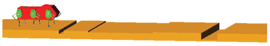
Comparative rough terrain crossing experiments were carried out to verify the comprehensive effectiveness of the whole controller. A comprehensive rough terrain was built with multistage slopes, a ditch, a fence, and two hillocks, as shown in Figure 23. The slope angles were 12, 25, and 12 degrees. The fence was 350 mm high. The ditch was 120 mm deep and the two hillocks were 120 mm high. The friction coefficient was set to be 0.9. Like the other experiments introduced above, a tripod gait and the free gait were both employed. The yaw angle comparison and the roll angle comparison are shown in Figure 24.

Rough terrain model.
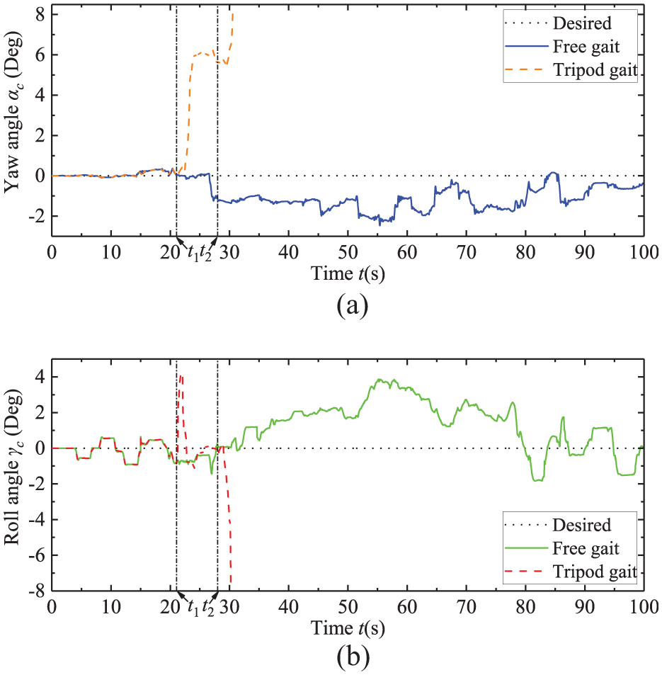
Results of the rough terrain crossing: (a) yaw angle comparison and (b) roll angle comparison.
At t1 = 21 s, leg 1 of the hexapod robot kicked the fence during the swinging status. As shown in Figure 24, the yaw and roll angles of the robot walking with the tripod gait fluctuated sharply. The robot failed to pass the fence and unstable motion state occurred. At t2 = 28 s, the second fence kicking occurred and the robot lost its stability thoroughly. During the whole process of walking with the tripod gait, the maximum absolute tracking errors of the yaw and roll angles were 8.15 and 7.78 degrees and their standard deviations were 2.49 and 1.01 degrees, respectively.
As a comparison, the yaw and roll angles could almost remain stable even when the robot came across the mutations on the terrain. Due to the obstacle negotiation method in the free gait controller, the robot passed the fence stably. After passing the fence, the robot could also deal with the remaining mutations and the slopes due to the free gait controller proposed. During the whole rough terrain walking process with the free gait, the maximum absolute tracking errors of the yaw and roll angles were 2.47 and 3.87 degrees and their standard deviations were 0.71 and 1.38 degrees, respectively. A significant motion improvement of the robot was obtained. It should be noticed that the forward direction of the robot was not parallel to the direction of the slope. The angle between the forward direction of the robot and the direction of the slope caused the roll angle fluctuation. This is a normal phenomenon and cannot be regulated only by gait changing.
The forward foot force comparison of leg 1 at t1 = 21 s is shown in Figure 25. It can be seen that at t1 = 21 s leg 1 kicked the fence during the swing status and the forward foot force became nonzero. Without any regulation of the gait, leg 1 kept “fighting against” the fence. The maximum absolute forward foot force was 26 kN. This unexpected interaction caused the large fluctuation of the robot body attitude. But, with the application of the free gait controller, a steady motion was ensured. The maximum absolute forward foot force reached 5 kN and got down to zero fast.

Forward foot force of leg 1.
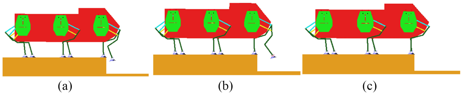
The whole free gait walking process is shown in Figure 26. The best support status was chosen automatically by the robot to cope with the local terrain mutations. Stable walking on the rough terrain was ensured due to the function of the free gait controller proposed.
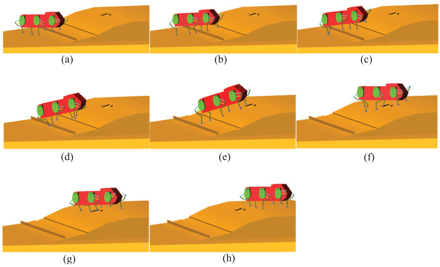
The rough terrain crossing process: (a) fence passing, (b) ditch passing, (c) three-legged support status → four-legged support status, (d) four-legged support status → five-legged support status, (e) hillock passing, (f) five-legged support status → four-legged support status, (g) four-legged support status → three-legged support status, and (h) walked to the top.
Conclusion and future work
In this article, the importance of heavy load robots walking on rough terrains with free gait is addressed. The main theoretical contribution of this article is the establishment of a free gait controller. The free gait controller designed for the heavy load hexapod robot used in this study mainly consists of two parts: a free gait planner and a gait regulator. The establishment of the free gait planner is based on a macro terrain recognition method proposed and a status searching method with stability and kinematic constraints considered. The gait regulator is established with switch rules for the leg motion status transition and the leg motion adjustment method for the ditch negotiation.
Detailed simulation experiments have been carried out to validate the effectiveness of the free gait controller. Simulation results show that the heavy load hexapod robot used in this article can choose the best walking gaits in time regarding the changes in the external environment. Motion performances are significantly improved compared with the commonly used tripod gait walking. Such results are very encouraging because the free gait controller proposed in this article has a good versatility and is not limited by different robot structures. Therefore, more applications of the free gait controller proposed can be expected.
In order to further improve the motion stability of the hexapod robot, the force equilibrium control method and body posture compensation method of the robot will be introduced into the controller in the future. Experiments on the real heavy load hexapod robot will be carried out.
Footnotes
Handling Editor: Emre Sariyildiz
Declaration of conflicting interests
The author(s) declared no potential conflicts of interest with respect to the research, authorship, and/or publication of this article.
Funding
The author(s) disclosed receipt of the following financial support for the research, authorship, and/or publication of this article: The authors gratefully thank the support of the National Natural Science Foundation of China (Grant Nos 61773139 and 61473015), the Natural Science Foundation of Heilongjiang Province, China (Grant No. F2015008), the State Key Laboratory of Robotics and System (HIT; Nos SKLRS201603C), and the Shenzhen Peacock Plan (No. KQTD2016112515134654).