
Abstract
The resonance failure of straight–curved combination pipes conveying fluid which are widely used in engineering is becoming a serious issue. But there are only few studies available on the resonance failure of combination pipes. The resonance failure probability and global sensitivity analysis of straight–curved combination pipes conveying fluid are studied by the active learning Kriging method proposed in this article. Based on the Euler–Bernoulli beam theory, the dynamic stiffness matrices of straight and curved pipes are derived in the local coordinate system, respectively. Then the dynamic stiffness matrix and characteristic equation of a straight–curved combination pipe conveying fluid are assembled under a global coordinate system. The natural frequency is calculated based on the characteristic equation. A resonance failure performance function is established based on the resonance failure mechanism and relative criterions. The active learning Kriging model based on expected risk function is introduced for calculating the resonance failure probability and moment-independent global sensitivity analysis index. The importance rankings of input variables are obtained with different velocities. According to the results, it is shown that the method proposed in this article provides a lot of guidance for resonance reliability analysis and anti-resonance design in combination pipes conveying fluid.
Keywords
Introduction
Pipes conveying fluid are widely used in aerospace, aircraft, nuclear, ocean, and petrification engineering. Because of the restriction on the construction room, the layout of combination pipes is always complicated such as L-shaped, U-shaped, and Z-shaped combination layouts rather than single straight pipes or curved ones. The L-shaped combination pipe is most especially used in engineering. The uncertainty of pipe and fluid will have an obvious effect on the natural frequency of the combination pipes. When the natural frequency is close to the excitation frequency, this will lead to the resonance failure. The straight–curved combination pipes have more complicated resonance failure relative to a single straight or curved pipe. It is essential and valuable to study the resonance reliability of a straight–curved combination pipe conveying fluid.
There has been a lot of research on the natural frequency of single straight or curved pipes considering fluid–structure interaction (FSI).1–6 MP Paidoussis 1 and MP Paidoussis and NT Issid 2 made a detailed study in his monographs on linear and nonlinear dynamics of the fluid-conveying pipes. HB Wen et al. 3 proposed a kinetic model of the straight–curved pipe conveying fluid. YJ Hu and WD Zhu 4 established a dynamic model of an extensible fluid-conveying curved pipe with an arbitrary undeformed configuration. N Egidi et al. 5 proposed a mathematical model for U-shaped geothermal heat exchangers based on the unsteady Navier–Stokes problems. Many researchers studied the in-plane and out-of-plane vibration modes of the curved pipe based on the total extensible and in-extensible assumption.6–9 The straight–curved combination pipes are always used in engineering. For the combination pipes, it is hard to establish the analytical solution, so the semi-analytical and numerical solutions such as finite element method, 10 dynamic stiffness matrix (DSM), 11 transfer matrix method (TMM), 12 substructure method, 13 and He’s vibration iteration method are employed. 14 The DSM method is independent of the element number. For a large-size element, the DSM method is also accurate, so the DSM is suitable for the vibration analysis of combination pipes. Koo used the Euler–Bernoulli beam theory to establish the DSM of a straight pipe, deduced the DSM of a curved pipe based on TMM, and then completed the combination of a straight and curved pipe. His method is directive for computing the straight–curved combination pipes. HL Dai et al. 15 used the TMM to establish the DSM of combination pipes by adding the axial combination force into the control equations of a straight pipe. Up to now, the methods for establishing the DSM of straight–curved combination pipes are always based on the straight pipe element, also called straight–straight combination. The straight–curved pipe element combination is not considered. Finite straight pipe elements are used for simulating the curved pipe combined with TMM. This will lead to the increase of dimensionality of DSM and the procedure is complex. Therefore, the accurate curved pipe elements are used for simulating the curved pipe in this study. In the global coordinate system, the whole DSM of straight–curved combination pipes is obtained, and then the natural frequency of the combination pipes can be computed.
The excitation of the pipes conveying fluid, especially aircraft pipes, is intense and wideband frequency, which will lead to resonance failure easily. Although there are a lot of works in dynamic research of pipes conveying fluid, there are only few studies researching the resonance failure of pipes; especially, there is only much less research on combination pipes. Because the combination pipes are widely used in engineering, it is valuable and essential to study the resonance failure of combination pipes conveying fluid. HB Zhai et al.
16
studied the dynamic reliability and local sensitivity analysis (LSA) of a straight pipe conveying fluid based on a refined response surface method, and the fluid profile in the pipe is uniform. AA Alizadeh et al.
17
used the Monte Carlo method to study the self-vibration and stability analysis of a fluid-conveying pipe. YL Li et al.
18
computed the reliability of subsea pipelines under spatially varying ground motions using subset simulation. The sensitivity analysis is used in many researches to identify the key parameters influencing the function of structures or systems.19–21 The sensitivity analysis has been applied to identify the key input parameters influencing the energy conversion factor of flexoelectric materials.
19
Hamdia et al.
20
presented a methodology for stochastic modeling of the fracture in polymer nanocomposites. Vu-Bac et al.
21
provided a sensitivity analysis toolbox consisting of a set of MATLAB functions that offer utilities for quantifying the influence of uncertainty input parameters on uncertain model outputs. LSA indices are defined as the partial derivate of the failure probability with respect to the distribution parameters of input variables. LSA indices can only reflect the local effect of the distribution parameters on the failure probability but cannot tell us how the uncertainty of the input variables affects the failure probability globally. The global sensitivity analysis (GSA) indices can help measure the effect of uncertainty of each input variable on the variance or the distribution of the model outputs of interest.
22
The GSA techniques include variance-based GSA, moment-independent GSA, and the screening method.23–27 In this article, the moment-independent GSA will be adopted to research the resonance failure. There are two main methods for calculating the moment-independent indices, the one is based on probability density function (PDF) proposed by Borgonovo et al.,23,24 Wei et al.,
25
Cui et al.,
26
and Wei et al.,
27
and the other one is based on cumulative distribution function (CDF) of the model output such as the PAWN method.
28
KM Hamdia et al.
28
have presented an improvement to the PAWN method that reduces the computational cost. Comparably, the moment-independent GSA indices, that is,
This article is organized as follows: section “Motion equations of combination pipes” introduces the DSM method and how to calculate the natural frequency of a combination pipe conveying fluid. Section “Resonance performance function” introduces the anti-resonance performance function of the combination pipe conveying fluid. Section “Moment-independent GSA” introduces the moment-independent GSA of resonance reliability on pipes conveying fluid. Section “The ALK model based on ERF” introduces the active learning Kriging (ALK) method based on expected risk function (ERF). Section “Example” gives an example of straight–curved combination pipes, and the resonance failure probabilities and moment-independent GSA indices with different velocities. Section “Conclusion” gives the conclusions.
Motion equations of combination pipes
The single straight pipe is shown in Figure 1. The Cartesian coordinates are built as shown in Figure 1.

The straight pipe conveying fluid.
Suppose that the damping of pipe materials and gravity are ignored, the fluid is in-viscous and incompressible. The pipe is based on Euler–Bernoulli beam theory. The FSI vibration equation of the straight pipe conveying fluid is1,29
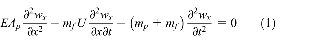


where
Equations (1)–(3) have a solution in the frequency domain as follows

where
Define the displacement state vector


According to equations (5) and (6), the dynamic relationship is

where
The curved pipe conveying fluid is shown in Figure 2. The curvilinear coordinates are built as shown in the figure.

The diagram of the curved pipe conveying fluid.
According to the research of Paidoussis, 1 for the curved pipe conveying fluid, ignoring pipe damping, the fluid is in-viscous and incompressible, ignoring the gravity; the three-dimensional (3D) dynamic equation of the curved pipe based on Euler–Bernoulli beam theory is


where
The general solution of equations (8)–(11) in the frequency domain is

where
Define the displacement state vector


Combining equations (13) and (14), the relationship can be rewritten as

where
The steps for calculating the natural frequency of straight–curved combination pipes are shown as follows:
Step 1. Discretize the straight–curved combination pipes into a single straight pipe element and a curved one, based on the Euler–Bernoulli beam theory, and build 3D vibration governing equations of the straight pipe and curved elements.
Step 2. Deduce discrete modes and DSM of the pipe elements based on the frequency dispersion relation.
Step 3. Assemble all straight pipe elements and the curved ones under a global coordinate system and establish the straight–curved combination pipe’s DSM.
Step 4. Considering the boundary conditions, build the characteristic equations of the straight–curved combination pipes. The natural frequency can be obtained by solving the characteristic equation.
Resonance performance function
To avoid resonance failure, the excitation frequency must be far away from the natural frequency of the straight–curved combination pipes conveying fluid. The resonance reliability analysis aims at estimating the resonance failure probability of the pipes conveying fluid.
In engineering, because of the uncertainty among materials, manufacturing, installation, and servicing, the excitation frequency, natural frequency, and vibration response are random variables. Based on the traditional design roles, if

where
Moment-independent GSA
The moment-independent GSA indices measure the relative importance of one input using the average shift between the unconditional and conditional PDFs of the model output when this input is fixed over its full distribution range.
22
The delta indices can be expressed as the accumulation of the difference between unconditional PDF
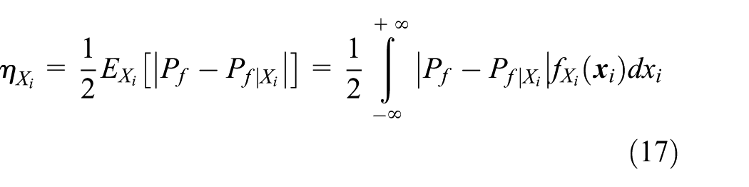
where
The absolute value in the above equation is difficult to compute, and it is equally transformed into square operation. 30 The modified global sensitivity indices on the failure probability can be expressed as follows

Because the resonance failure performance function is implicit, the response is hard to obtain. The Monte Carlo simulation method is used to calculate the failure probability

Compute the error of estimate by
The GSA focuses on measuring the effects of the uncertainty of each input variable on the variance or distribution parameters of the failure probability and deciding how to reduce the failure probability by decreasing the uncertainty of the input variables. By decreasing the uncertainty of the input variables with high moment-independent indices, we can achieve the most reduction of failure probability. By ignoring the uncertainty of the input variables with small moment-independent indices, we can reduce the dimensionality and simplify the procedure of anti-resonance optimization design.
The ALK model based on ERF
Because the resonance failure performance function is complex and implicit, the computational cost of the traditional Monte Carlo method is high and time consuming. To solve this problem, the approximation method such as support vector machines, 31 neural networks, 32 polynomial chaos expansions, 33 and Kriging model is introduced to approximate the implicit performance function which improves the computational efficiency greatly. The Kriging model method is widely adopted because of its high simulation accuracy. The ALK model means the Kriging model constructed by adding new training points probably located in the region of interest and updating the Kriging model. Through this iterative process, a large portion of the training points will be in the region of interest rather than throughout the design space.34–36 The ALK model can further improve the accuracy.
The predicted value

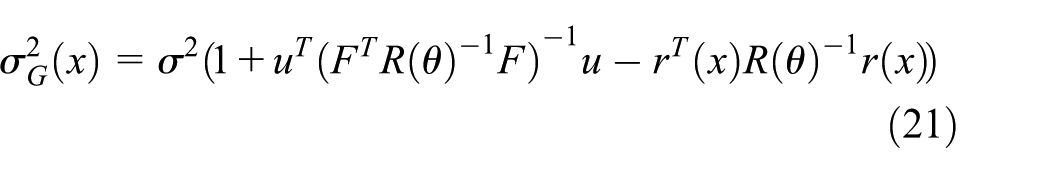
where

The ALK model is established in the DACE toolbox of MATLAB.
37
The global optimization algorithm adopted in this article is the modified dividing rectangles algorithm for calculating the parameter
To improve the ability of predicting the objective function’s plus or minus sign, the point with the largest risk of being wrongly predicted would be picked out and added into the DoE. The ability of predicting the objective function’s sign would be improved mostly. The ERF is a learning function used to identify this point with a high risk.
The Kriging model provides a predicted value

The indicator

In the case of

And the expectation of risk can be expressed as
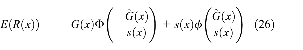
The ERF also called learning function of the predicted value

where
The ERF is a measurement of the potential risk of a point at which the sign of the performance function can be expected to be changed form positive to negative. The point maximizing ERF should be added to the DoE. ERF indicates the probability that the predicted value is different from the real value, that is, the larger the value of ERF is, the more likely it is that the real value changes from positive to negative or from negative to positive. In addition, the points where the ERF values are relatively large are generally the points near the limit state surface and the points with large Kriging variances. Therefore, these ERF maximum points should be added to the DoE to improve the accuracy of the Kriging model. The ALK solution based on ERF for

The flow diagram of the ALK method proposed in this article.
Here N = 20 is the number of initial samples for establishing the initial Kriging model. And m = 105 is the number of candidate points for selecting samples by ERF. Some candidate points (m*) will be selected to calculate the resonance failure and moment-independent GSA index through the Monte Carlo method based on the Kriging model. The total call count number of the performance function is N + m*. And X denotes the n-dimensional input vector which has the maximum ERF, which is not a number, but is an input vector, X = (x1, x2, …, xn), where n is the number of total input variables.
Example
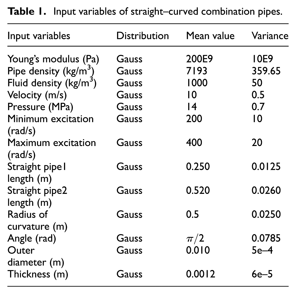
Combining two straight pipes and one curved pipe, the L combination pipe is obtained as shown in Figure 4. The information of geometry and materials is listed in Table 1. The boundary condition is clamped–clamped supported at both ends.
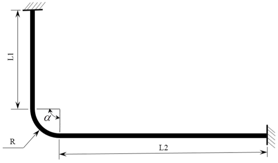
The L combination pipe diagram.
Input variables of straight–curved combination pipes.
Natural frequency
The natural frequency of L combination pipe is calculated, and the results are presented in Figure 5. According to Figure 5, it is shown that, in the natural frequency of L combination pipe, there exist two closed frequencies, which is because the pipe model in this article is 3D Euler–Bernoulli beam, not only the in-plane vibration but also the out-of-plane vibration.

Natural frequency of straight–curved combination pipes.
Figure 6 shows the relationship of the natural frequency with the velocity. From Figure 6, it is shown that, with the increase of velocity, the natural frequency of the combination pipe decreases until the natural frequency falls to zero suddenly. This is because the centrifugal and Coriolis force items in the vibration equations increase along with the increase of velocity. When the velocity is

First four natural frequencies with the increasing fluid velocity.
Resonance reliability
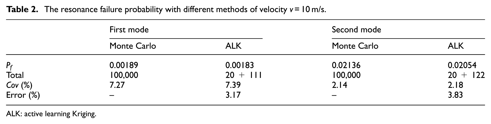
The resonance failure probability is calculated by the ALK method and compared with the value calculated by the Monte Carlo method as shown in Table 2.
The resonance failure probability with different methods of velocity v = 10 m/s.
ALK: active learning Kriging.
Along with the increasing velocity, the first- and second-order resonance failure probabilities are listed in Table 3. It is shown that, along with the increasing velocity, the first-order resonance failure probability is getting smaller and the second-order resonance failure probability is getting larger. It is because the natural frequency is getting smaller along with the increasing velocity, the resonance failure area between the minimum excitation frequency and natural frequency is smaller, and the resonance failure area between the maximum excitation frequency and natural frequency is getting larger. The results calculated by the method proposed in this article coincide with the analytical results.
The resonance failure probability with different velocities.

Moment-independent GSA
When the velocity is
Table 4 presents the importance measurement. It is shown that when the velocity
The moment-independent GSA indices of input variables.

GSA: global sensitivity analysis.
Considering the input variables

The failure probability along with the increasing variance of
Conclusion
Based on the Euler–Bernoulli beam theory, the accurate curved pipe model is used for establishing the DSM. Then all straight pipe elements and the curved ones are assembled under a global coordinate system. The natural frequency can be calculated based on the characteristic equation. After establishing the performance function of resonance failure, the ALK model based on ERF is used to calculate the resonance failure probability and moment-independent GSA index. The method proposed in this article is guided for resonance reliability analysis and GSA.
First, the natural frequencies with different velocities are calculated. It is found that, along with the increasing velocity, the natural frequency is getting smaller. When the velocity reaches to the critical velocity, the first-order natural frequency of the combination pipe becomes zero and buckling instability occurred. Second, the ALK model based on ERF is used for calculating the resonance failure probability and moment-independent indices. Along with the increasing velocity, the first-order resonance failure probability is getting smaller, while the second-order resonance failure probability is getting larger. The result coincides with the theoretical analysis. Finally, the importance ranking is obtained from the moment-independent indices. The variance of input variables with high moment-independent index were changed from 0.03 to 0.06. The resonance failure probability is getting larger along with the increasing variance of the input variables with high moment-independent indices. The larger the moment-independent indices, the greater the resonance failure probability increase caused by changing the variance. If the input variable with larger indices is controlled strictly, the resonance failure probability can be reduced much more than the other variables. From the results, the method proposed in this article is meaningful for resonance failure analysis of straight–curved combination pipes and is referential for other combination pipes.
For the future research work, the resonance failure performance function will be improved, while the traditional performance function does not consider the multi-order resonance failure. The second point of future study is to improve the calculation efficiency. Because the performance function is implicit, the time cost for calculation is huge, especially for sensitivity analysis. Therefore, a more efficient solving method is needed.
Footnotes
Handling Editor: Mohammad Arefi
Declaration of conflicting interests
The author(s) declared no potential conflicts of interest with respect to the research, authorship, and/or publication of this article.
Funding
The author(s) received no financial support for the research, authorship, and/or publication of this article.