
Abstract
A steady-state boundary layer flow analysis of a non-Newtonian magnetic fluid over a shrinking sheet was studied. The boundary layer thickness and the velocity distribution in the layer were studied under the conditions of a uniform magnetic field normal to the shrinking sheet and/or a vertical uniform mass suction across the sheet. The similarity transformation method was used to transform the governing partial differential equations to ordinary differential equations. The shooting method with Newton’s algorithm and Runge–Kutta integration method were used to obtain the solutions of the equations. The results showed that the variation of the flow velocity profiles in the boundary layer was significant, the thickness of the boundary layer was thinner, and the skin friction coefficient was bigger for either shear thinning or shear thickening magnetic fluids under the conditions of a stronger magnetic field or a larger mass suction effect.
Introduction
The fluid flow varies due to electromagnetic interference, if the fluid contains metal particles that belong to the scope of application of the conductive fluid. The external magnetic field environment might impact flow or heat transfer effect in stretching or shrinking the product, for example, iron and steel casting, plastic injection molding, film production, and other processes. Therefore, it is necessary to further study the characteristics of the conductive fluid.
By the use of numerical methods, Andersson et al. 1 propose that magnetic field makes the boundary layer thin and increases skin friction. Chiam 2 explores numerical solution of velocity change impacted in the boundary layer in the transverse magnetic field and finally proves the initial condition values speculated by Crocce’s method inferred guess get closer. Andersson et al. 3 investigate the transient boundary layer velocity field. Stretched flat surface is obtained through numerical methods to derive solutions of transient parameters and power index. Yürüsoy 4 found that boundary layer development is similar with Newtonian fluid under shear thinning conditions and the boundary layer thickness increases with the power parameters under shear thickening conditions.
Miklavčič and Wang 5 investigate the solution of velocity boundary layer in one-dimensional and two-dimensional (2D) models. Wang 6 found that shrinking sheet often present and flow in the opposite direction of contraction in boundary layer, which hinders the heat transfer and mass transfer effects.
Amkadni et al. 7 numerically solve the inhalation, injection parameters and magnetic parameters on the impact of velocity boundary layer. Fang 8 derive similar equation based on the assumption of boundary layer by suction parameters and the power of speed-related parameters β. Sajid and Hayat 9 determine convergence polynomial solution using homotopy analysis method based on the suction parameters and magnetic field strength parameter. Mahapatra et al. 10 investigate the impact of shear-stress factor by the ratio of the fluid velocity and the extend speed. Kumaran et al. 11 investigate the magnetic parameters, suction parameters, injection parameters, linear parameters and nonlinear parameters, and then summed up five different individual cases. Fang and Zhang 12 identify closed-form exact solution of similar equations by numerical analysis. Fang et al. 13 discuss transient behavior of the external viscous fluid in the boundary layer when the plane contracts. Noor et al. 14 use Adomian decomposition method with Padé approximants program and obtain results similar to Sajid and Hayat. 9 Fang and Zhong 15 investigate the tablet contraction condition in the case of various speeds in viscosity fluids using Navier–Stoke equation. Merkin and Kumaran 16 investigate the transient influence of magnetic field on Newtonian fluid when it produced velocity boundary layer at the time of contraction of flat plate, and use numerical method to obtain continuous equation.
Bhatti et al. 17 found that velocity of the fluid for large values of magnetic parameter and porosity parameter is reduced. Radiation effects show an increase in the temperature profile, whereas thermal slip parameter shows converse effect. Mohyud-Din et al. 18 use Buongiorno’s model to investigate the heat and mass transfer of a nanofluid over a suddenly moved flat plate. Bhatti et al. 19 adopts a new numerical method to solve the stagnation-point flow problem over a permeable stretching/shrinking sheet through porous media. Reddy CS et al. 20 examine the magnetohydrodynamic boundary layer flow with heat and mass transfer of Williamson nanofluid over a stretching sheet with variable thickness and variable thermal conductivity under the radiation effect. Rashidi et al. 21 show that the thermal boundary layer thickness gets decreased with increasing Prandtl number. Brownian motion plays an important role in improving thermal conductivity of the fluid.
This article will explore the impact of boundary layer of conductive Newtonian fluid and non-Newtonian fluid flown over a shrinking sheet in a fixed magnetic field environment.
Mathematical method
Model representation
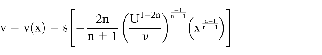
In the condition of the presence of a fixed uniform magnetic field in a vertical plate direction, non-Newtonian fluid containing tiny magnetic molecules, when planar is contraction, this article analyzes the boundary layer flow field generated by the surface. Figure 1 is a schematic representation of a flat shrink. It is assumed that shrinkage to the plate center is only in x direction, so this will take half of the model as discussed. Figure 2 is a schematic representation of the physical model. The plate length is L, uniform thickness is T, and L>>T represents thin plate. External environment exits a fixed magnetic B in y direction and flat shrink at a speed u = –Ux in x direction, thus generated a boundary layer flow on the surface. The surface of boundary layer flow field exits suction velocity v(x) in y direction, speed in x direction outside of the boundary layer flow field is

The schematic representation of flat shrinking.

The schematic representation of the half-range physical model.
Governing equations
This study uses the following assumptions:
The flow is a 2D steady laminar flow.
The fluid is incompressible and is a conductive power-law viscous fluid.
The fluid density, magnetic field, and other physical properties are constant.
When plate shrinks, the mass suction effect is on the plate surface.
The magnetic Reynolds number with the present conductive fluid material is much less than 1.0.
In a 2D incompressible steady-state conductive flow, the mass conservation equation is

By using Newton’s second law of motion, we can derive the momentum conservation equation as follows

where

where kinematic viscosity
The study assumed that the plate shrinks in the negative x direction, at a speed u = –Ux at


where v(x) is assumed to be derived by a similar conversion method and helps to simplify similar equation. s is the suction parameter and n is the power-law index.
Governing equation’s similar conversion
A similar conversion method transforms the 2D mass conservation and momentum conservation equations of partial differential equations into ordinary differential equations, followed by a numerical method to solve it. Assume that stream function ψ and a similar variable η can be expressed as follows


where
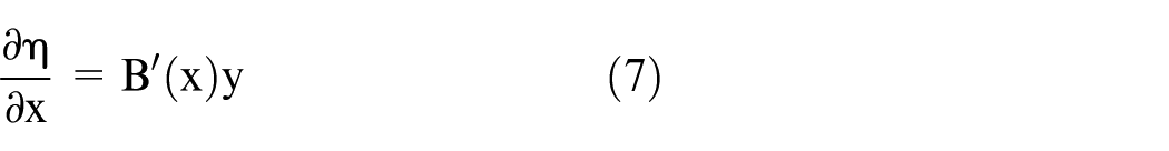
By derivating equation (6) for x and y, we get

Using equation (5), we can derive velocity u and v as follows


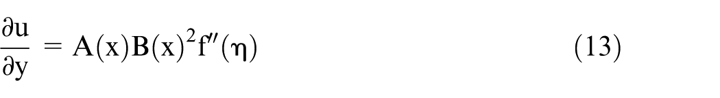
The partial differential equation of u, v for x and y, respectively, can computed as follows


Equations (11) and (12) equal zero, representing that the similarity transformation parameters has met continuous equation (1). Then other items in the momentum conservation equation (3) with similar conversion parameter indicates

By substituting equations (9)–(14) in the momentum conservation equation (3), we can derive a similar equation

In order to eliminate the constants in similarity equation, assume that the constant items in equation (15) is


where
By transposition from the equation (16), we can obtain


By transposition and integration, we get
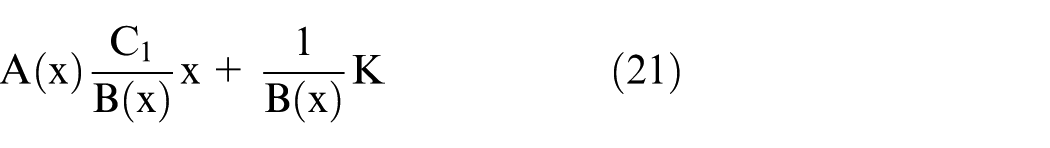
where K is constant. By substituting equation (19) into equation (21) and ignoring the constant term K, we obtain
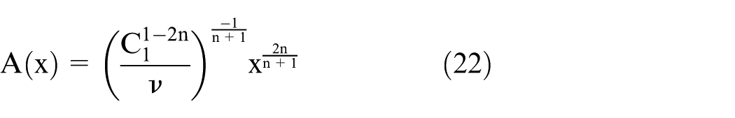
Then substituting equation (22) into equation (19), we can obtain
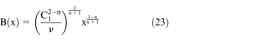
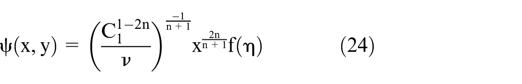
Substituting equations (22) and (23) in equations (5) and (6), respectively, can obtain the stream function and similar conversion factor as follows

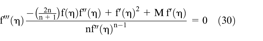
By a similar conversion method, the momentum conservation equation (3) can be rewritten as
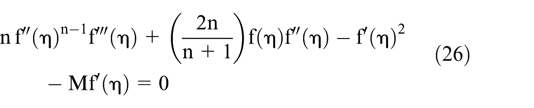
where power-law index (n) is represents as: when
By substituting
where the suction parameter is a dimensionless mass suction velocity.
Equation’s analytical solution
Miklavčič and Wang 5 get similar equation as

When the power-law index n = 1, the fluid is a Newtonian fluid. Without considering the magnetic field and the magnetic fluid, equation (26) can be expressed as

So then from Miklavčič and Wang
5
gets when
The equation (26) is expressed as
By the boundary condition

And two sets of analytical solution are obtained as follows

and

where K is constant. The results of equation (32) and that of numerical analysis are the same.
Numerical procedure
Governing equations of this study has been converted into a third-order nonlinear ordinary differential equation by similar conversion method. This article uses the shooting method with second-order Newton’s method to find the initial conditions
Numerical methods process
The process of the numerical calculation is shown in Figure 3.
The first, given boundary conditions, wherein the initial condition of the suction parameter f(0) is 0–6. Second-order initial conditions
Give integration interval of f(η) in solving equation, so that η satisfies the boundary condition when
The error value analyzing the convergence is given as
To solve similarity equations, when the difference between the values
To archive and to plot from obtaining data are done.

The flow chart of numerical methods.
Program and numerical verification
The fluid being used is a Newtonian fluid and is not subject to magnetic interference in the situation, namely power-law index n = 1, the magnetic field strength parameter M = 0 in similar equation, equation (26) can be reduced to

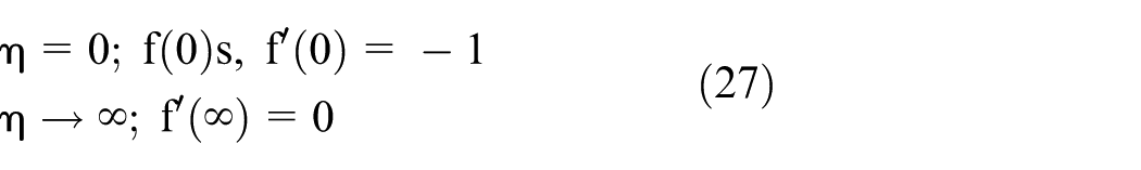
This ordinary differential equation with boundary conditions in equation (27), it can be solved.
Figure 4 is the relationship curve between

The velocity gradient profiles f″ (0) versus s for n = 1 and M = 0 with different values of β.
Fluid used here is a conductive Newtonian fluid and is subject to magnetic interference in the situation, namely power-law index n = 1, the magnetic field strength parameter M is constant in similar equation, equation (25) can be reduced to

This ordinary differential equation with boundary conditions in equation (26), it can be solved.
This article assumes that the fluid (n = 1, M = 0, 1) has the same conditions similar to a study by Fang and Zhang.
12
Using numerical methods we can solve equation (35) and explore the physical meaning of partial solutions. Figure 5 is the relationship curve between

The velocity gradient profiles f″(0) versus s for n = 1 and M = 0 with different values of M.
Results and discussions
Discussion on numerical operations
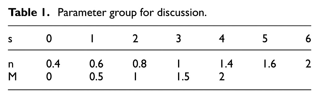
Explored parameter group are shown in Table 1. In the case of boundary conditions equation (27) using numerical methods for the equation (26) obtained the graph of
Parameter group for discussion.
Figures 6 and 7 show the velocity profiles for M = 2 and several values of s: (a) n = 0.6, (b) n = 1 and (c) n = 1.6. From the figure, it can be found whether the fluid is a conductive Newtonian fluid or a conductive non-Newtonian fluid.
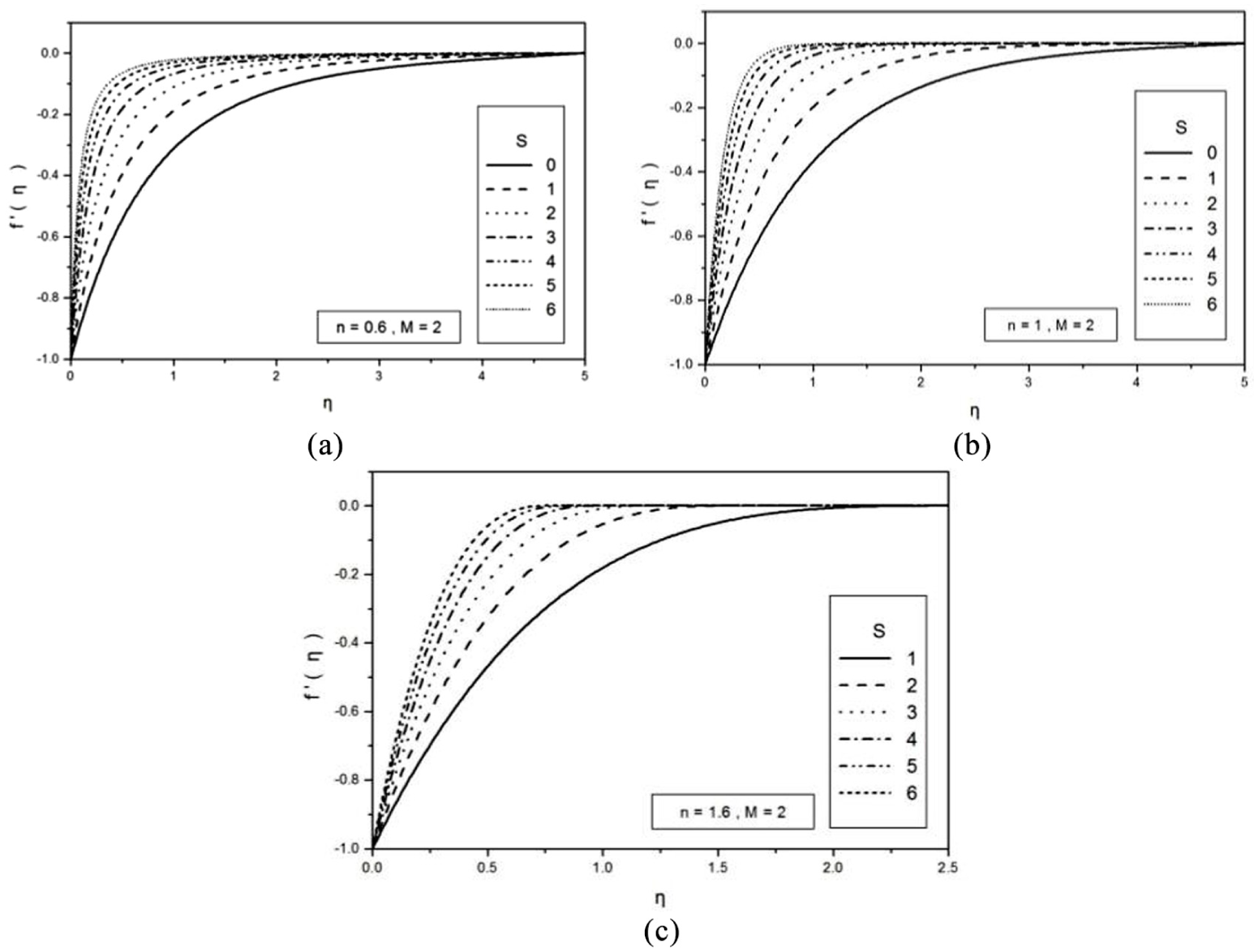
The velocity profiles for M = 2 and several values of s: (a) n = 0.6, (b) n = 1, and (c) n = 1.6.

The velocity gradient profiles for M = 2 and several values of s: (a) n = 0.6, (b) n = 1, and (c) n = 1.6.
Figures 8 and 9 show the velocity profiles for several values of M: (a) n = 0.6, s = 4, (b) n = 1, s = 3 and (c) n = 1.6, s = 2. From the figure it can be found whether the fluid is a conductive Newtonian fluid or a conductive non-Newtonian fluid.

The velocity profiles for several values of M: (a) n = 0.6, s = 4; (b) n = 1, s = 3; and (c) n = 1.6, s = 2.

The velocity gradient profiles for several values of M: (a) n = 0.6, s = 4; (b) n = 1, s = 3; and (c) n = 1.6, s = 2.
Discussion on skin friction coefficient
In addition,

Figure 10 shows the velocity gradient profiles for several values of M: (a) n = 0.4, (b) n = 1 and (c) n = 2. Found from the figure, when the M is larger, the solved interval trend appears extended to the left, which represents increasing M, and in the case of smaller s, the similar solution of velocity boundary layer can also be obtained, and it has the same trend similar to the results of Fang and Zhang.
12
The trend of the curve can be found, when s value is, M is larger, and
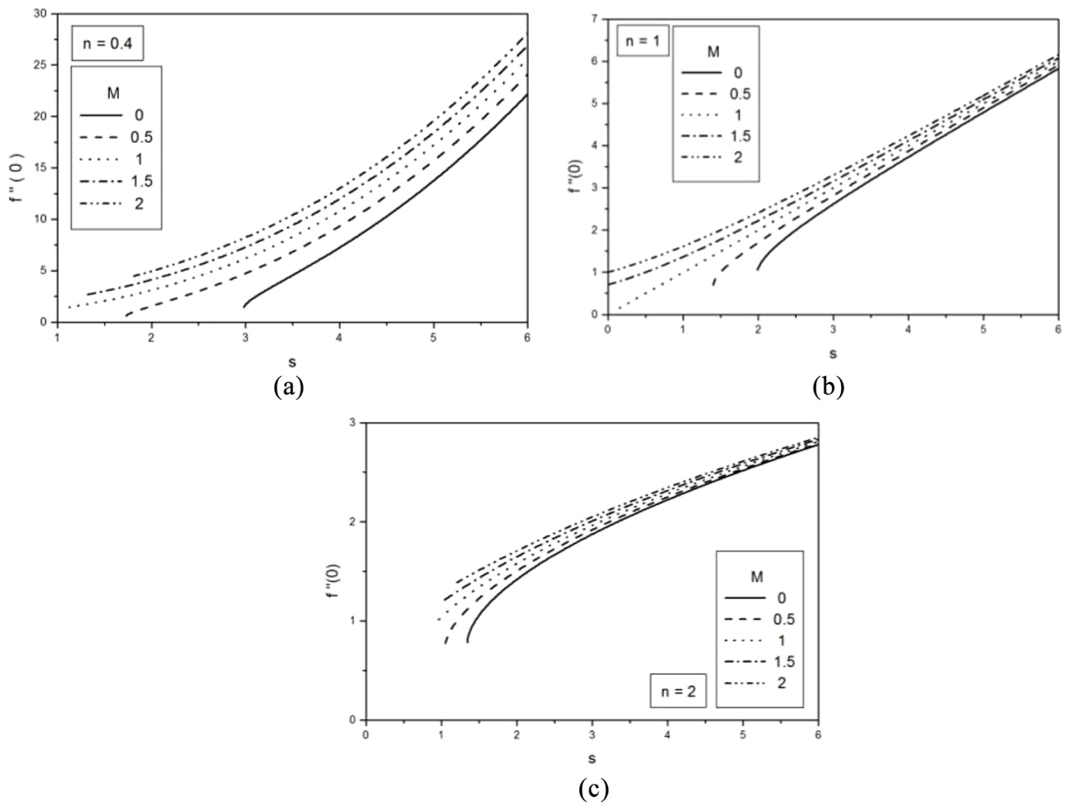
The velocity gradient profiles for several values of M: (a) n = 0.4, (b) n = 1, and (c) n = 2.
Figure 11 shows velocity gradient profiles for several values of n: (a) M = 0, (b) M = 1 and (c) M = 2. The figure found that the solved interval in the process of transform from n < 1 into n = 1 and then into n > 1 is gradually moved downward in the case of fixed M value.

The velocity gradient profiles for several values of n: (a) M = 0, (b) M = 1, and (c) M = 2.
On observing the whole curve, it can be understood that the interval of the solved solution moves downward. The gradually decreased f″(0) value represents
Discussion on dimensionless boundary layer thickness
This article uses similar conversion method for solving the dimensionless velocity distribution on boundary layer. When
Figure 12 shows diagram of boundary layer thickness under M = 0 and 2, corresponding to different values of s. In the case of a fixed M, greater n has smaller
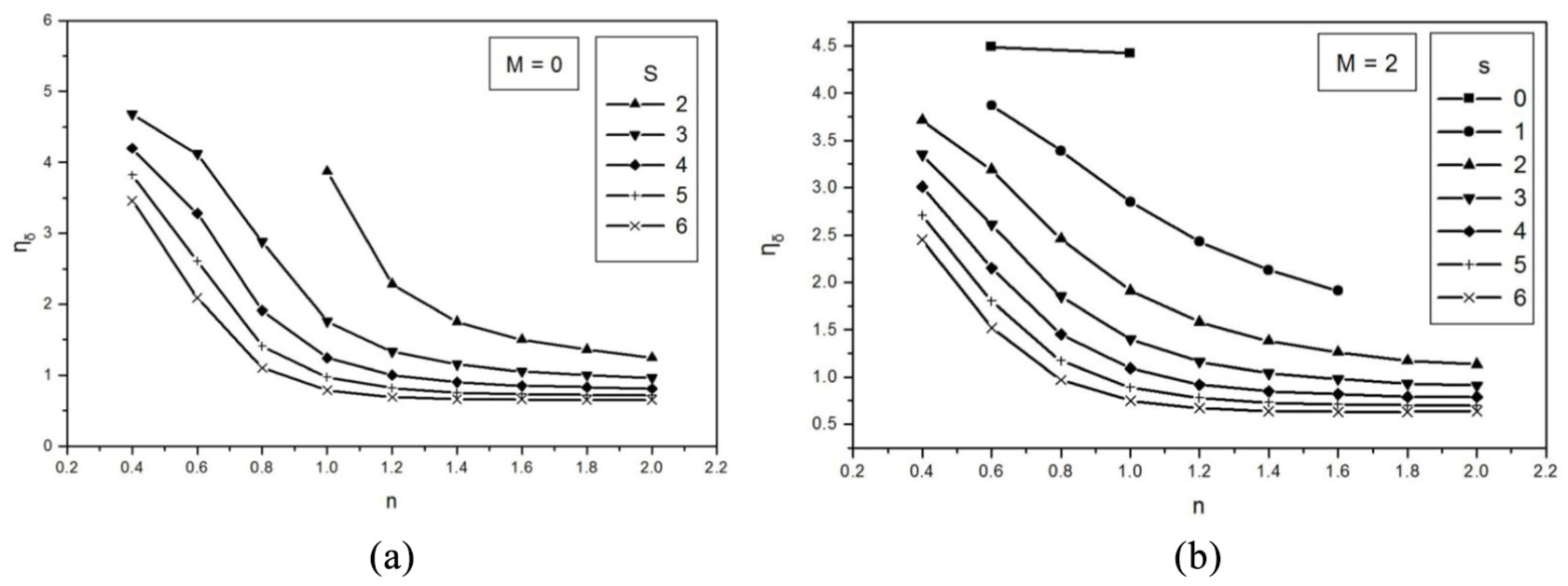
The boundary layer thickness profiles for several values of s: (a) M = 0 and (b) M = 2.
Figure 13 shows diagram of boundary layer thickness under s = 3 and 6, corresponding to different values of M. In the case of a fixed s, greater n has smaller

The boundary layer thickness profiles for several values of M: (a) s = 3 and (b) s = 6.
Conclusion
When the magnetic field strength parameter or the suction parameters increase, similar equation whether the fluid is conductive Newtonian fluid or conductive non-Newtonian fluids, governing equation in the numerical calculation reach all the fast convergence conditions. Among them was severely affected by suction parameters.
When the magnetic field strength parameter or suction parameters increases, the shear stress of flat surface becomes large, among which was severely affected by suction parameters. The shear stress of shear thinning conductivity non-Newtonian fluid is greater than that of conductivity Newtonian fluid and is greater than that of shear thickening conductivity non-Newtonian fluid.
When the magnetic field strength parameters increase or the suction parameters increase, whether the fluid is a Newtonian fluid conductive or conductive non-Newtonian fluid, the thickness of boundary layer decreases.
Under the same magnetic field strength parameters and suction parameters, the thickness of the boundary layer of shear thinning conductivity non-Newtonian fluid is greater than that of conductivity Newtonian fluid and is greater than that of shear thickening conductivity non-Newtonian fluid.
Footnotes
Appendix 1
Handling Editor: Xiao-Jun Yang
Declaration of conflicting interests
The author(s) declared no potential conflicts of interest with respect to the research, authorship, and/or publication of this article.
Funding
The author(s) received no financial support for the research, authorship, and/or publication of this article.