Sage Journals: Discover world-class research

Abstract

A multi-dimensional lumped element model of a long non-rotating rod that moves on a slick surface with both dynamic and static Coulomb friction is outlined. The rod is accelerated to a constant velocity, and the free end of the rod experiences the effect of stick and slip. This article describes a new modeling approach, where the model is able to switch between different linear semi-analytical sub-models, depending on how much of the rod is moving. Fundamental understanding of the stick–slip effect is revealed, and a potential shortcoming of the model is also discussed. The model is computationally effective and may be suitable for real-time applications in, for instance, oil-well drilling.

Keywords

Coulomb friction lumped element models drillstring dynamics

Introduction

The complex phenomenon named dry friction occurs when two surfaces are in contact with each other. Experiments indicate dependence on a number of parameters such as normal force, combination of materials, roughness, temperature, sliding speed, and even acceleration. Depending on the application, the friction models may have functional relations with velocity, time lag, or dwell time, or include pre-slip displacement. In Berger’s study,¹ a multi-disciplinary review of the plethora of friction models is given, while in Feeny et al.’s study,² a historical review on dry friction and the stick–slip effect is given.

However, in many applications, the original model by Charles Augustin Coulomb is often a sufficient approximation. The sliding Coulomb friction force is directed opposite to the sliding motion, and the magnitude is equal to the normal force multiplied by a kinematic friction coefficient. When the surfaces stick together, the static Coulomb friction force can have any direction, and the magnitude can be anything between zero and the static friction coefficient multiplied by the normal force. Mathematically, this model is therefore highly non-linear.

A common way to model the Coulomb friction force is to use a functional relationship with velocity, that is, $μ (v) N$ , where N is the normal force and $μ (v)$ is the friction coefficient that is a function of the velocity v. The function is typically a continuous step function such as the inverse tangent function with various parameters (see Zhao et al.³). This modeling approach is believed to be robust when the static friction coefficient is not high compared to the kinetic friction coefficient.⁴

Another way to model the Coulomb friction is to work directly with the discontinuous relations and switch between models when the surfaces go from stick to slip, and vice versa. The sub-models are typically linear and can sometimes be solved analytically. In Cull and Tucker,⁵ torsional vibrations of an oil-well drillstring are analyzed with both modeling types. It was shown that the models compare well, when the kinematic friction coefficient is not small compared to the static friction coefficient, and the viscous damping is relatively small.

A switching modeling approach with sub-models that are linear with analytic or semi-analytic solutions is well suited for real-time applications such as control algorithms, fault detection, and parameter estimation. This is therefore the model of choice in this article.

Similar to Cull and Tucker,⁵ our motivation is related to oil-well drilling where kilometer-long pipes are frequently run into or pulled out of wellbores. The models in Cull and Tucker⁵ contain only two degrees of freedom and describe important physical phenomena but are not appropriate for the complex geometries of real wells.

Fortunately, a number of semi-analytical models for both the axial and torsional movements of an oil-well drillstring in both vertical and deviated wellbores are developed. In Hovda,⁶ axial vibrations of a vertical wellbore are described, while the axial vibrations of a deviated wellbore while reaming are outlined in Hovda.⁷ A model for the torsional vibrations is presented in Hovda.⁸

These semi-analytical models are particularly suited for a switching model approach, since they can include three-dimensional wellbore geometries and non-homogeneous pipe sizes. For the sake of exposure, we have focused our study to a straight rod with uniform thickness, with homogeneously distributed friction forces along the rod. This model can easily be generalized in many ways, but this is outside the scope of this article. The goal of this article is merely to describe and validate the model with a variety of computational experiments that are physically intuitive.

The general model is outlined in the next section, and computational experiments are given in the section after that. The model relies on various assumptions, which are defined when needed, and furthermore discussed and summarized in the “Discussion” section. The article is concluded in the last section.

Dynamic model of a long non-rotating rod that is moving on a surface with Coulomb friction

We consider a rod of length L that is modeled as a set of n blocks that are connected by n spring elements (see Figure 1). The inclination angle of the rod is denoted by $θ$ . A one-dimensional coordinate system along the rod with positive direction downward is introduced. The first block is hanging from the first spring which is attached to a point that is denoted by $Q (t)$ , and the origo of the coordinate system is chosen so that $Q (0) = 0$ .

Figure 1.

Schematic view of the model of the rod that is sliding on the surface. The rod is modeled as a set of n blocks with masses denoted by $m_{i}$ . These masses are connected to n springs, where the spring constants are denoted by $k_{i}$ . The surface is shown as the line that the rod or blocks are sliding on.

The center point on each block is denoted as $X_{i} (t)$ , where t is time. When all springs are not in compression and not in tension, the distance between the points is equal to h. We define $q_{i} (t)$ as $X_{i} (t) - ih$ and the physical state of the drillstring at any time is therefore uniquely defined by the generalized coordinates, $q_{i} (t) s$ .

Newton’s second law on every block gives

\begin{matrix} 0 = m_{1} {\overset{\cdot\cdot}{q}}_{1} - m_{1} g \cos (θ) + k_{1} (q_{1} - Q) - \\ k_{2} (q_{2} - q_{1}) + c_{1} {\overset{\cdot}{q}}_{1} - R_{1} \\ 0 = m_{i} {\overset{\cdot\cdot}{q}}_{i} - m_{i} g \cos (θ) + k_{i} (q_{i} - q_{i - 1}) - \\ k_{i + 1} (q_{i + 1} - q_{i}) + c_{i} {\overset{\cdot}{q}}_{i} - R_{i} for 2 \leq i \leq n - 1 \\ 0 = m_{n} {\overset{\cdot\cdot}{q}}_{n} - m_{n} g \cos (θ) + k_{n} (q_{n} - q_{n - 1}) + c_{n} {\overset{\cdot}{q}}_{n} - R_{n} \end{matrix}

(1)

where for block i, $m_{i}$ is the mass and $k_{i}$ is the spring constant of the spring that is located above the block. The gravity constant is g and the $c_{i} s$ are some constants related to damping. This could, for instance, be the viscous damping that is discussed in Hovda.⁶ Finally, the Coulomb friction forces are denoted by the $R_{i} s$ .

Coulomb friction forces

Coulomb friction states that the friction force between two sliding surfaces is proportional to the normal force with direction that opposes the motion. Moreover, two surfaces stick together unless the force between the surfaces exceeds the normal force multiplied by the static friction coefficient. The static friction coefficient is typically higher than dynamic friction coefficient. The static friction is considered to arise as a result of surface roughness features across multiple length scales at solid surfaces.

The kinematic Coulomb friction on block i is $R_{i} = d_{2, i} μ_{k, i} m_{i} g \sin (θ)$ , where $μ_{k, i}$ is the kinematic Coulomb friction constant and $d_{2, i}$ is plus one when ${\overset{\cdot}{q}}_{i} \leq 0$ and minus one when ${\overset{\cdot}{q}}_{i} > 0$ . For convenience in this model, $\overset{\cdot}{Q}$ is used, instead of ${\overset{\cdot}{q}}_{i}$ , and therefore we have $d_{2} = d_{2, i}$ . Moreover, the static Coulomb friction on block i is $R_{i} = d_{2} μ_{s, i} m_{i} g \sin (θ)$ , where $μ_{s, i}$ is the static Coulomb friction constant. More precisely

\begin{matrix} R_{i} = {\begin{matrix} S F_{i} & for | S F_{i} | \leq μ_{s, i} m_{i} g \sin (θ) \\ and {\overset{\cdot}{q}}_{i} = {\overset{\cdot\cdot}{q}}_{i} = 0 \\ d_{2} μ_{k, i} m_{i} g \sin (θ) & else \end{matrix} \end{matrix}

where $S F_{i}$ is the sum of all other forces than the Coulomb friction forces, that is

\begin{matrix} S F_{1} = - m_{1} g \cos (θ) + k_{1} (q_{1} - Q) - k_{2} (q_{2} - q_{1}) \\ S F_{i} = - m_{i} g \cos (θ) + k_{i} (q_{i} - q_{i - 1}) - k_{i + 1} (q_{i + 1} - q_{i}) \\ for 2 \leq i \leq n - 1 \\ S F_{n} = - m_{n} g \cos (θ) + k_{n} (q_{n} - q_{n - 1}) \end{matrix}

(2)

In this article, situations when the rod is starting from rest and being pulled out are discussed. In this case, it makes sense to make the assumption that if a block i is stalled in static friction, that is, $| S F_{i} | \leq μ_{s, i} m_{i} g \sin (θ)$ and ${\overset{\cdot}{q}}_{i} = 0$ , then all blocks below this block are also stalled, that is, ${\overset{\cdot}{q}}_{j} = 0$ for $j \geq i$ . In the case when the pulling out motion is stopping, the first element stops before the elements below are stopped. The current model can be generalized to include this, but this is outside the scope of this article.

Consequently, in the situations discussed in this article, we have $n_{d}$ blocks that are moving and $n_{s}$ blocks that are not moving due to static friction. Therefore, $n_{d} + n_{s} = n$ , where $n_{s}$ is zero when the whole rod is moving.

At a certain time, a model for the rod involves a sub-model of the top $n_{d}$ blocks, while the bottom $n_{s}$ blocks rest at its initial conditions. This sub-model is valid until either ${\overset{\cdot}{q}}_{n_{d}}$ becomes zero or ${\overset{\cdot}{q}}_{n_{d} + 1}$ becomes different than zero. In the case of pulling the rod out from an initial rest position, the model will switch between different sub-models until the whole rod is moving. In the first sub-model, $n_{d}$ will be zero and then $n_{d}$ will increase to n.

In order to find a model for when block number $n_{d} + 1$ will start to move (provided that $n_{d} \neq n$ ), we investigate $| S F_{n_{d} + 1} | = μ_{s, nd + 1} N_{n_{d} + 1}$ . It is clear that $S F_{n_{d} + 1}$ can only be close to $- μ_{s, n_{d} + 1} m_{n_{d} + 1} g \sin (θ)$ when running in and that $S F_{n_{d} + 1}$ can only be close to $μ_{s, n_{d} + 1} m_{n_{d} + 1} g \sin (θ)$ when running out. We therefore conclude that block number $n_{d} + 1$ will start to move (provided that $n_{d} \neq n$ ) when $S F_{n_{d} + 1} = d_{2} μ_{s, nd + 1}$ $m_{n_{d} + 1} g \sin (θ)$ . Mathematically, this is

\begin{matrix} Q = (1 + \frac{k_{2}}{k_{1}}) q_{1} - \frac{k_{2}}{k_{1}} q_{2} - \\ \frac{m_{1} g \cos (θ) + d_{2} μ_{s, 1} m_{1} g \sin (θ)}{k_{1}} \\ for n_{d} = 0 \\ q_{n_{d}} = (1 + \frac{k_{n_{d} + 2}}{k_{n_{d} + 1}}) q_{n_{d} + 1} - \frac{k_{n_{d} + 2}}{k_{n_{d} + 1}} q_{n_{d} + 2} - \\ \frac{m_{n_{d} + 1} g \cos (θ) + d_{2} μ_{s, n_{d} + 1} m_{n_{d} + 1} g \sin (θ)}{k_{n_{d} + 1}} \\ for 1 \leq n_{d} \leq n - 2 \\ q_{n_{d}} = q_{n} - \frac{m_{n} g \cos (θ) + d_{2} μ_{s, n} m_{n} g \sin (θ)}{k_{n}} \\ for n_{d} = n - 1 \end{matrix}

(3)

This concludes the criterion for moving to a model with $n_{d} + 1$ blocks. The model with $n_{d} - 1$ blocks is changed when ${\overset{\cdot}{q}}_{n_{d}} = 0$ .

Mathematical model for $n_{d}$ elements

We follow the same procedure as in Hovda⁶ and develop equation (1) into a system of $n_{d}$ coupled second-order ordinary differential equations. The matrix form is

\begin{matrix} M \overset{\cdot\cdot}{q} + C \overset{\cdot}{q} + K q - g - r = f (t) \end{matrix}

(4)

where all matrices are square of the size $n_{d} \times n_{d}$ and $q$ is a vector of size $n_{d}$ . Here, $M$ and $C$ are diagonal matrices with the $m_{i} s$ and the $c_{i} s$ on the respective diagonals. The tridiagonal matrix $K$ is equal to

\begin{matrix} [\begin{matrix} k_{1} + k_{2} & - k_{2} & \dots & 0 & 0 \\ - k_{2} & k_{2} + k_{3} & \dots & 0 & 0 \\ 0 & - k_{3} & \dots & 0 & 0 \\ ⋮ & ⋮ & ⋱ & ⋮ & ⋮ \\ 0 & 0 & \dots & - k_{n_{d} - 1} & 0 \\ 0 & 0 & \dots & k_{n_{d} - 1} + k_{n_{d}} & - k_{n_{d}} \\ 0 & 0 & \dots & - k_{n_{d}} & k_{n_{d}} + k_{n_{d} + 1} \end{matrix}] \end{matrix}

where $k_{n + 1}$ is defined to be zero. The elements of $g$ are constants of the form $m_{i} g \cos (θ)$ , and the vector $r$ has the elements $d_{2} μ_{k, i} m_{i} g \sin (θ)$ when $i \leq n_{d} - 1$ and $r_{n_{d}} = d_{2} μ_{k, n_{d}} m_{n_{d}} g \sin (θ) + k_{n_{d} + 1} q_{n_{d} + 1}$ . The first element of $f (t)$ is equal to $k_{1} Q (t)$ , while the others are zero.

We make the coordinate transformation $q = y + K^{- 1} (g + r)$ where the inverse of $K$ is given analytically in Hovda.⁹ The constant shift from $q$ to $y$ corresponds to the vector of strains from the tension and compression forces that are acting on the drillstring when the driving force has been zero for a long time.

Then, equation (4) takes the form

\begin{matrix} M \overset{\cdot\cdot}{y} + C \overset{\cdot}{y} + K y = f (t) \end{matrix}

(5)

which means that when all derivatives are zero and the driving force is zero, all $y_{i} s$ are also zero. We choose a new timescale which is $τ = (c_{s} / L) t$ , where $c_{s}$ is the speed of sound in the rod (typically steel). We define E as the Young’s modulus and $ρ_{s}$ as the density of the material in the rod, so that $c_{s}^{2} = E / ρ_{s}$ . This means that equation (5) can be written as

\begin{matrix} A_{1} \overset{\cdot\cdot}{y} + \frac{n c_{s}}{E \hat{a}} C \overset{\cdot}{y} + n^{2} A_{2} y = \frac{nL}{E \hat{a}} f (τ) \end{matrix}

(6)

where $A_{1}$ is a diagonal matrix with $a_{i} s$ on its diagonal and $A_{2}$ is a tridiagonal matrix that is similar to $K$ , where the $k_{i} s$ are substituted by the $a_{i} s$ . The parameter $a_{i}$ is the cross-sectional area of the $i th$ block, divided by $\hat{a}$ , which is the geometric mean of all n (and not $n_{d}$ ) cross-sectional areas. Note that $k_{i} = E \hat{a} a_{i} / h$ . In the case when $n_{d} = n$ , the determinant of $A_{1}$ is one.

This is a linear system of first-order ordinary differential equations

\begin{matrix} {\overset{\cdot}{y}}_{b} = A_{b} y_{b} + f_{b} (τ), where \\ y_{b} = [\begin{matrix} y \\ \overset{\cdot}{y} \end{matrix}], A_{b} = [\begin{matrix} 0 & 1 \\ - n^{2} {A_{1}}^{- 1} A_{2} & - \frac{n c_{s}}{E \hat{a}} {A_{1}}^{- 1} C \end{matrix}] and \\ f_{b} (τ) = [\begin{matrix} 0 \\ \frac{nL}{E \hat{a}} {A_{1}}^{- 1} f \end{matrix}] \end{matrix}

which has the solution by using integrating factors

\begin{matrix} y_{b} = \int_{0}^{τ} \exp ((τ - u) A_{b}) f_{b} du + \exp (τ A_{b}) y_{b} (0) \\ = U (\exp (τ E)) U^{- 1} *_{τ} f_{b} (τ) + U \exp (τ E) U^{- 1} y_{b} (0) \end{matrix}

(7)

where $y_{b} (0)$ is the concatenation of the initial conditions $y (0)$ and $\overset{\cdot}{y} (0)$ . Moreover, the operation $*_{τ}$ is convolution with respect to $τ$ on the interval zero to $τ$ , and the matrix exponential is decomposed by eigenvalue decomposition such that $A_{b} = UE U^{- 1}$ . From Tisseur and Meerbergen,¹⁰ we have that the system has two times $n_{d}$ finite eigenvalues that appear in conjugate pairs.

This decomposition contains all the parameters in the model, which limits the possibilities of detection of unknown parameters. We have therefore found a trick to avoid this by assuming that $C = (c_{1} / a_{1}) A_{1}$ . This is the same as assuming that the system is proportionally damped. By taking an eigenvalue decomposition ${A_{1}}^{- 1} A_{2} = VD V^{- 1}$ , we can approximate $A_{b}$ by

\begin{matrix} A_{b} = [\begin{matrix} 0 & 1 \\ - n^{2} VD V^{- 1} & - c 1 \end{matrix}] \end{matrix}

where

\begin{matrix} c = \frac{n c_{s} c_{1}}{E a_{1} \hat{a}} \end{matrix}

We define $ω_{i} = n \sqrt{D_{ii}}$ , $ζ_{i} = c / (2 ω_{i})$ , and the damped angular frequency $ω_{d, i} = ω_{i} \sqrt{1 - ζ_{i}^{2}}$ . By solving the characteristic equation of $A_{b}$ , we get that

\begin{matrix} E = [\begin{matrix} Λ_{1} & 0 \\ 0 & Λ_{2} \end{matrix}] \end{matrix}

where the diagonal elements of the diagonal matrices $Λ_{1}$ and $Λ_{2}$ are $- c / 2 + i ω_{d, i}$ and $- c / 2 - i ω_{d, i}$ , respectively. Moreover, by solving that $A_{b} U = UE$ we get that

\begin{matrix} U = [\begin{matrix} V & V \\ V Λ_{1} & V Λ_{2} \end{matrix}] \end{matrix}

and the inverse of this block matrix is

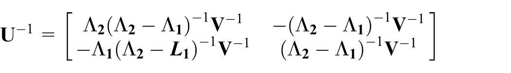
\begin{matrix} U^{- 1} = [\begin{matrix} Λ_{2} {(Λ_{2} - Λ_{1})}^{- 1} V^{- 1} & - {(Λ_{2} - Λ_{1})}^{- 1} V^{- 1} \\ - Λ_{1} {(Λ_{2} - L_{1})}^{- 1} V^{- 1} & {(Λ_{2} - Λ_{1})}^{- 1} V^{- 1} \end{matrix}] \end{matrix}

which is easily verified by checking that $U^{- 1} U = 1$ . From equation (7), we see that it is interesting to inspect the upper-left and the upper-right block matrices of $U \exp (τ E) U^{- 1}$ . They are equal to

\begin{matrix} V (Λ_{2} \exp (τ Λ_{1}) - Λ_{1} \exp (τ Λ_{2})) {(Λ_{2} - Λ_{1})}^{- 1} V^{- 1} \end{matrix}

and

\begin{matrix} V (- \exp (τ Λ_{1}) + \exp (τ Λ_{2})) {(Λ_{2} - Λ_{1})}^{- 1} V^{- 1} \end{matrix}

respectively. We therefore have the full solution

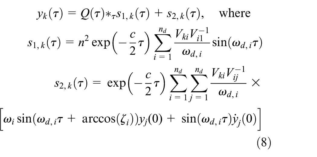
\begin{matrix} y_{k} (τ) = Q (τ) *_{τ} s_{1, k} (τ) + s_{2, k} (τ), where \\ s_{1, k} (τ) = n^{2} \exp (- \frac{c}{2} τ) \sum_{i = 1}^{n_{d}} \frac{V_{ki} V_{i 1}^{- 1}}{ω_{d, i}} \sin (ω_{d, i} τ) \\ s_{2, k} (τ) = \exp (- \frac{c}{2} τ) \sum_{i = 1}^{n_{d}} \sum_{j = 1}^{n_{d}} \frac{V_{ki} V_{ij}^{- 1}}{ω_{d, i}} \times \\ [ω_{i} \sin (ω_{d, i} τ + \arccos (ζ_{i})) y_{j} (0) + \sin (ω_{d, i} τ) {\overset{\cdot}{y}}_{j} (0)] \end{matrix}

(8)

By noting that the derivative of $\exp (- c τ / 2) \sin (ω_{d, i} τ)$ is equal to $- ω_{i} \exp (- c τ / 2)$ $\sin (ω_{d, i} τ - \arccos (ζ_{i}))$ and that the derivative of $\exp (- c τ / 2) \sin (ω_{d, i} τ + \arccos (ζ_{i}))$ is equal to $- ω_{i} \exp$ $(- c τ / 2) \sin (ω_{d, i} τ)$ , we see that the derivatives are given by

\begin{matrix} {\overset{\cdot}{y}}_{k} (τ) = Q (τ) *_{τ} {\overset{\cdot}{s}}_{1, k} (τ) + {\overset{\cdot}{s}}_{2, k} (τ), where \\ {\overset{\cdot}{s}}_{1, k} (τ) = - n^{2} \exp (- \frac{c}{2} τ) \sum_{i = 1}^{n_{d}} \frac{V_{ki} V_{i 1}^{- 1}}{\sqrt{1 - ζ_{i}^{2}}} \times \\ \sin (ω_{d, i} τ - \arccos (ζ_{i})) \\ {\overset{\cdot}{s}}_{2, k} (τ) = - \exp (- \frac{c}{2} τ) \sum_{i = 1}^{n_{d}} \sum_{j = 1}^{n_{d}} \frac{V_{ki} V_{ij}^{- 1}}{\sqrt{1 - ζ_{i}^{2}}} \times \\ [ω_{i} \sin (ω_{d, i} τ) y_{j} (0) + \sin (ω_{d, i} τ - \arccos (ζ_{i})) {\overset{\cdot}{y}}_{j} (0)] \end{matrix}

(9)

Similarly, we see that the accelerations are given by

\begin{matrix} {\overset{\cdot\cdot}{y}}_{k} (τ) = Q (τ) *_{τ} {\overset{\cdot\cdot}{s}}_{1, k} (τ) + {\overset{\cdot\cdot}{s}}_{2, k} (τ), where \\ {\overset{\cdot\cdot}{s}}_{1, k} (τ) = n^{2} \exp (- \frac{c}{2} τ) \sum_{i = 1}^{n_{d}} \frac{ω_{i} V_{ki} V_{i 1}^{- 1}}{\sqrt{1 - ζ_{i}^{2}}} \times \\ \sin (ω_{d, i} τ - 2 \arccos (ζ_{i})) and \\ {\overset{\cdot\cdot}{s}}_{2, k} (τ) = \exp (- \frac{c}{2} τ) \sum_{i = 1}^{n_{d}} \sum_{j = 1}^{n_{d}} \frac{ω_{i} V_{ki} V_{ij}^{- 1}}{\sqrt{1 - ζ_{i}^{2}}} \times \\ [ω_{i} \sin (ω_{d, i} τ - \arccos (ζ_{i})) y_{j} (0) + \\ \sin (ω_{d, i} τ - 2 \arccos (ζ_{i})) {\overset{\cdot}{y}}_{j} (0)] \end{matrix}

(10)

The challenges with solving this set of equations are to compute the convolutions $Q (τ) *_{τ} s_{1, k} (τ)$ , $Q (τ) *_{τ} {\overset{\cdot}{s}}_{1, k} (τ)$ , and $Q (τ) *_{τ} {\overset{\cdot\cdot}{s}}_{1, k} (τ)$ . However, they can be solved analytically by demanding that Q is a polynomial. By using the rule of partial integration m times, we see that

\begin{matrix} τ^{m} *_{τ} s_{1, k} (τ) = m! (D^{- (m + 1)} s_{1, k}) (τ) - \\ \sum_{j = 0}^{m} \frac{m!}{j!} (D^{- (m - j + 1)} s_{1, k}) (0) τ^{j} \\ τ^{m} *_{τ} {\overset{\cdot}{s}}_{1, k} (τ) = m! (D^{- (m)} s_{1, k}) (τ) - \\ \sum_{j = 0}^{m} \frac{m!}{j!} (D^{- (m - j)} s_{1, k}) (0) τ^{j} \\ τ^{m} *_{τ} {\overset{\cdot\cdot}{s}}_{1, k} (τ) = m! (D^{- (m - 1)} s_{1, k}) (τ) - \\ \sum_{j = 0}^{m} \frac{m!}{j!} (D^{- (m - j - 1)} s_{1, k}) (0) τ^{j} \end{matrix}

(11)

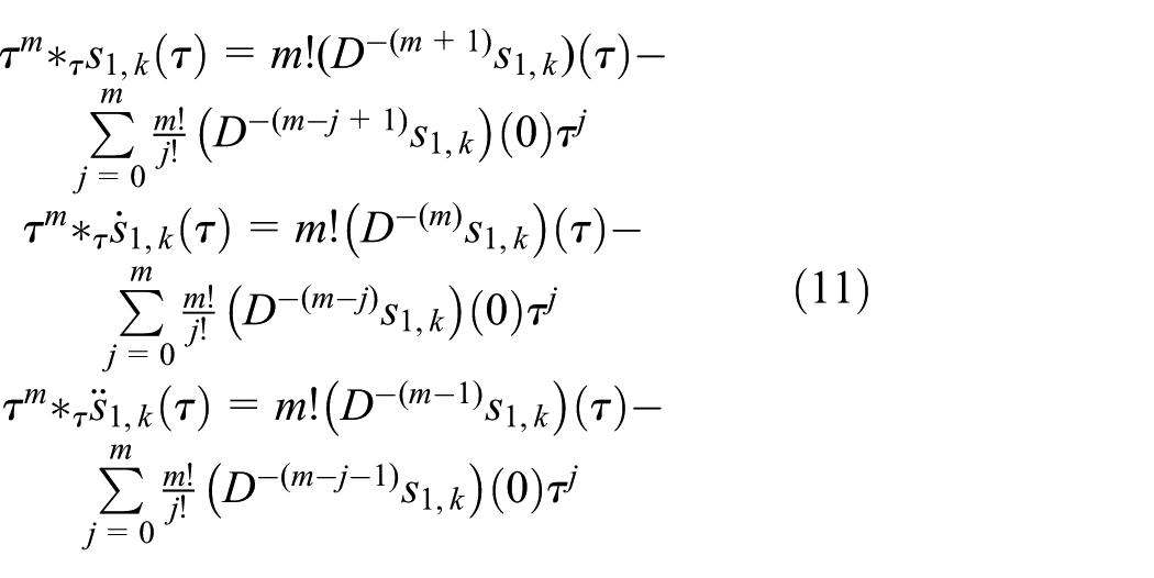
Here, when m is positive, the operator $(D^{m} f) (τ)$ denotes the $m th$ derivative of f with respect to $τ$ . When m is negative, $(D^{m} f) (τ)$ denotes the $- m th$ antiderivative with respect to $τ$ . Also, $(D^{0} f) (τ) = f (τ)$ .

By noting that the $m th$ derivative of $\exp (- c τ / 2) \sin (ω_{d, i} τ)$ is equal to $(- ω_{i})^{m} \exp (- c τ / 2)$ $(- c τ / 2) \sin (ω_{d, i} τ - m \arccos (ζ_{i}))$ and that the $m th$ antiderivative of $\exp (- c τ / 2) \sin (ω_{d, i} τ)$ is equal to $(- ω_{i})^{- m} \exp (- c τ / 2) \sin (ω_{d, i} τ + m \arccos (ζ_{i}))$ , we get that

\begin{matrix} (D^{m} s_{1, k}) (τ) = n^{2} \exp (- \frac{c}{2} τ) \sum_{i = 1}^{n_{d}} \frac{{(- ω_{i})}^{m} V_{ki} V_{i 1}^{- 1}}{ω_{d, i}} \times \\ \sin (ω_{d, i} τ - m \arccos (ζ_{i})) \end{matrix}

(12)

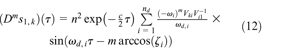
This means that when Q is a polynomial, we have an analytic solution for movement anywhere in the rod. Moreover, it is important to note that we can also use piecewise polynomials which allow for a rich variety of movements at the top. An obvious recommendation is that the derivative should be continuous over the breaks.

Computational experiments

Although the outlined model describes a rod with varying cross-sectional areas, where both the static and the dynamic Coulomb friction coefficients can vary anywhere along the rod, we focus our attention on the most basic cases.

We keep all masses and springs equal and keep both the dynamic and static Coulomb friction coefficients constant along the rod. As seen by equations (1) and (4), the effect of the angle $θ$ has two effects, one is related to the coordinate transform between $q$ and $y$ and the other is basically a factor of $\cos (θ)$ in front of the Coulomb friction coefficients. We have therefore decided to only use $θ = π / 2$ , which means that the rod is laying on a horizontal surface. For simplicity, we let the length of the rod be equal to how far the speed of sound travels in 1 s. This means that $τ = t$ .

In the computation experiments, we vary the static Coulomb friction coefficients $μ_{s}$ , the dynamic Coulomb friction coefficients $μ_{k}$ , and also the linear friction coefficient c.

In order to get some physical intuition about the linear friction coefficient c, we assume that the rod is sliding inside an outer pipe that is filled with water with viscosity of 1 cP. If we also assume that the diameter of the outer pipe is twice the diameter of the rod and that the weight of the rod is 25 kg per meter, then an approximation of the linear friction coefficient is

\begin{matrix} c = \frac{2 π L μ c_{s}}{E a_{1} \hat{a}} {(\frac{1 + α^{2}}{1 - α^{2}} \ln (α^{- 1}) - 1)}^{- 1} \\ = \frac{2 π μ}{ρ_{s} a_{1} \hat{a}} {(\frac{5}{3} \ln (2) - 1)}^{- 1} = 0.0016 \end{matrix}

according to Hovda,⁶ where $α$ is the diameter fraction and $μ$ is the viscosity.

Furthermore, in this article, we discuss driving forces that are limited to this piecewise polynomial

\begin{matrix} Q (τ) = {\begin{matrix} 0 & for τ \leq 0 \\ - \frac{V}{2 τ_{acc}} τ^{2} & for 0 < τ \leq τ_{acc} \\ - V (τ - \frac{τ_{acc}}{2}) & for τ_{acc} < τ \end{matrix} \end{matrix}

which describes when the rod is accelerated to the speed V in the period from $τ = 0$ to $τ = τ_{acc}$ . Moreover, $\overset{\cdot\cdot}{Q} (t)$ is a square function of the form

\begin{matrix} \overset{\cdot\cdot}{Q} (τ) = {\begin{matrix} 0 & for τ \leq 0 \\ - \frac{V}{τ_{acc}} & for 0 < τ \leq τ_{acc} \\ 0 & for τ_{acc} < τ \end{matrix} \end{matrix}

Note that by taking the second derivative of equation (6) with respect to $τ$ , we see that the relation between ${\overset{\cdot\cdot}{y}}_{k} (τ)$ and $\overset{\cdot\cdot}{Q} (τ)$ is exactly the same as the relation between $y_{k} (τ)$ and $Q (τ)$ . Since the mass and stiffness are uniform in this setting, we realize by consulting Hovda¹¹ that the accelerations anywhere in the rod will be a sum of square waves, one traveling upward and one traveling downward. We can also expect a Gibbs-like ringing in the acceleration signals, which is dependent on the choice of n.

In this article, we consider three initial conditions:

Rest, but previous pullout: This is $q (0) = K^{- 1} (g + r)$ , where $d_{2} = 1$ and $\overset{\cdot}{q} (0) = 0$ . This means that the positions of the blocks are the same as if the rod was previously pulled out slower and slower till it finally stopped.

Rest, but previous run in: This is $q (0) = K^{- 1} (g + r)$ , where $d_{2} = - 1$ and $\overset{\cdot}{q} (0) = 0$ . This means that the positions of the blocks are the same as if the rod was previously ran in slower and slower till it finally stopped.

Rest, but previous rotation: This is $q (0) = K^{- 1} (g)$ and $\overset{\cdot}{q} (0) = 0$ . This means that the positions of the blocks are the same as if the rod was previously rotated, that is, $r = 0$ .

Basic experiment that describes the undamped motion with equal static and dynamic Coulomb friction coefficients

In this case, the rod starts at rest from previous pullout. In the beginning $n_{d} = 0$ , and incrementally more blocks start to move and finally $n_{d} = n$ . We have $c = 0$ , $μ_{s} = μ_{k} = 0.35$ , $V = 1$ , and $τ_{acc} = 4$ .

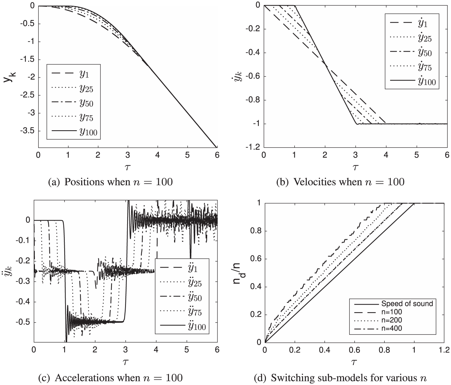
In Figure 2, we see the positions, the velocities, and the accelerations of the rod at various places, where $n = 100$ . As expected, the first block follows $Q (t)$ closely. In order to describe the movement of the other blocks, we study the acceleration plot in Figure 2(c). Because of the initial step in acceleration, the acceleration of the $n th$ block becomes a square wave with a period of four time units. It takes one time unit to start the movement, which is the time sound that needs to move to the other end of the rod. Then, ${\overset{\cdot\cdot}{y}}_{n}$ jumps from zero to twice the amplitude of the step, that is, $- 2 V / τ_{acc} = - 0.5$ . It stays at this level when the sound travels back and forth, and at $τ = 3$ , it jumps back to zero. All of this is in accordance with the result of Hovda.¹¹

Figure 2.

(a–c) The positions, velocities, and acceleration at various places in the rod. The parameters are $c = 0$ , $μ_{s} = μ_{k} = 0.35$ , $V = 1$ , and $τ_{acc} = 4$ . (d) How the model switch from $n_{d}$ equals zero to n for various n. For large n, we see that the switching is approaching the speed of sound. (a) Positions when n = 100, (b) velocities when n = 100, (c) accelerations when n = 100, and (d) switching sub-models for various n.

At $τ = 4$ , the acceleration at the top jumps back to zero, which sets of a new square wave that cancels out the previous square wave. This is a consequence of choosing $τ_{acc}$ to be equal to four. Note that we also see the Gibbs-like ringing signal, whose frequency is dependent on n as discussed in Hovda.¹¹ The acceleration anywhere else in the rod is a bit more complex, but it helps to understand that they are essentially a sum of a sound wave moving upward (or left) and a sound wave moving downward (or right). This is discussed more thoroughly in Hovda.¹¹

In Figure 2(d), we see a plot that describes how the model is switching between various sub-models. As expected, when the rod is at rest, $n_{d}$ is equal to zero and as the rod starts to move, $n_{d}$ increases to n. Since $μ_{s} = μ_{k}$ and the previous movement was being pulled out, a point in the rod starts to move when the sound wave reaches that point. In this case, movement of the $n th$ block should start at exactly one time unit, which is in accordance with Figure 2(a)–(c). However in Figure 2(d), we see that the $n th$ block actually starts to move at about $τ = 0.78$ . The movement is very small before $τ = 1$ . Moreover, since the speed of sound is constant, the graph in Figure 2(d) should also be linear, but we see that the movement of the first block happens earlier.

This is believed to be a consequence of the way we model the rod. Movement of the first block starts faster than the speed of sound, since the sub-model has too few blocks to incorporate this effect. Sub-models that contain more blocks are more accurate and the propagation speed becomes the speed of sound. By increasing n, we see in Figure 2(d) that this inaccuracy is reduced, that is, the movement at the bottom approaches the logical limit of one. However, the problem will always occur in the first few blocks.

Experiment that describes the undamped motion when the static is larger than the dynamic Coulomb friction coefficient

In this case, the rod also starts at rest from previous pullout. In the beginning $n_{d} = 0$ , and incrementally more elements start to move and finally $n_{d} = n$ . Different from the experiment in this section, we have $μ_{s} = 0.55$ , while the other parameters are unchanged, that is, $μ_{k} = 0.35$ , $c = 0$ , $V = 1$ , and $τ_{acc} = 4$ .

In Figure 3(a), we show the velocities at various places in the rod for $n = 100$ . The graphs are similar to Figure 2(b), when $μ_{s} = μ_{k} = 0.35$ . However, movement starts later, because the sum of the forces that are acting on the blocks has to overcome the static Coulomb friction forces (which are larger than the kinematic Coulomb friction forces). In Figure 3(c), we see a close-up of the movement of the first four blocks. We see that the movement of a block accelerates much faster than $Q (τ)$ , but this acceleration reduces and actually becomes negative when this block has moved sufficiently far away from the next block. Eventually, the next block cuts loose and a new wave of motions happens. In Figure 3(d), we see that increasing n to 200 has the effect of increasing the frequency of these wave motions. This is an interesting result, because if we are modeling a slick pipe with a number of blocks and springs, we get these wave motions that are a consequence of dividing the rod into a set of springs and masses. For a perfect slick pipe, these motions will not happen in reality.

Figure 3.

(a) The velocities in various places of the rod, when the parameters are $c = 0$ , $μ_{k} = 0.35$ , $μ_{s} = 0.55$ , $V = 1$ , $τ_{acc} = 4$ , and $n = 100$ . Close-up plots for the first four blocks are given in (c) and (d) for n equal to 100 and 200, respectively. We see plots regarding the switching between various sub-models for various n in (b). (a) Velocity overview n = 100, (b) switching sub-models, (c) velocity close-up n = 100, and (d) velocity close-up n = 200.

In Figure 3(b), we see the effect of switching between sub-models. For the first block, it does not start to move before the rod has moved long enough to overcome the static friction force. This is slower than the speed of sound. The movement of the last block is limited by the speed of sound. Increasing n has the effect of driving the $n th$ block movement closer to the speed of sound.

Experiment that describes the damped motion for various acceleration lengths

In this case, the rod also starts at rest from previous pullout. Different from the experiment in this section, we have $c = 0.0016$ and we vary $τ_{acc}$ . To be precise, $μ_{s} = μ_{k} = 0.35$ , $c = 0.016$ (10 times more viscous than the example given in this section), $V = 1$ , and $n = 100$ .

In Figure 4(a), we see the velocities at various parts of the rod when the acceleration length is one time unit. In the undamped case (not shown), the acceleration at the bottom is a sum of two square waves, where the second square wave has opposite amplitude and starts one time unit later. Therefore, the acceleration at the bottom is zero in first time unit, $- 2 V$ in the second time unit, zero in the third time unit, and finally $2 V$ in the last time unit. The solid graph in Figure 4(a) shows a damped version of this, meaning that the amplitude of the square acceleration waves is damped. The shapes of the other graphs can be understood in the same manner.

Figure 4.

The derivative of the position in various places in the rod for various acceleration lengths. The other parameters are $c = 0.016$ , $μ_{s} = μ_{k} = 0.35$ , $V = 1$ , and $n = 100$ . It is clear that stick–slip may occur if the acceleration phase is less than two time units. (a) Velocities when τ_acc = 1, (b) velocities when τ_acc = 2, (c) velocities when τ_acc = 5, and (d) velocities when τ_acc = 6.

The important result of Figure 4(a) and (b) is that the velocity can reach zero when $τ_{acc} \leq 2$ . When the velocity anywhere in the rod reaches zero, we can have the stick–slip effect, which will be described more in this section. We added the damping coefficient in this experiment to avoid the complexity of explaining stick–slip at this point in the article.

Figure 4(c) and (d) is added to show that the movement in the rod continues if the acceleration phase exceeds four time units. We therefore suggest that if one wants to avoid vibrations, the acceleration phase should be about four time units. In a practical system with damping and possibly non-homogeneous pipe size, one should aim for four times the first eigenfrequency.

Experiment that describes the effect of stick–slip

In this case, the rod also starts at rest from previous pullout. We let the acceleration phase be one time unit, that is, $τ_{acc} = 1$ . Moreover, we have $μ_{s} = 0.55$ , $μ_{k} = 0.35$ , $c = 0.0016$ , $V = 1$ , and $n = 100$ .

Figure 5(a) and (b) shows the movement of the rod in various places. Stick–slip occurs when $4 < τ < 5$ , and this is shown in Figure 5(c), where we see that about the last 30% of the rod are experiencing stick–slip. In Figure 5(d), we have reduced both V and $μ_{s} - μ_{k}$ by a factor of 10. Notice the similarity between Figure 5(b) and (d). This is explained as follows.

Figure 5.

Movements in various places in the rod in the case of stick–slip. The other parameters are $c = 0.0016$ , $μ_{s} = 0.55$ , $μ_{k} = 0.35$ , $V = 1$ , and $n = 100$ . (a) Positions when $V = 1$ and $μ_{s} - μ_{k} = 0.2$ , (b) velocities when $V = 1$ and $μ_{s} - μ_{k} = 0.2$ , (c) model switching when $V = 1$ and $μ_{s} - μ_{k} = 0.2$ , and (d) velocities when $V = 0.1$ and $μ_{s} - μ_{k} = 0.02$ .

By investigation equation (3), we see that the $y_{j} (0) s$ in equation (8) are dependent on the difference $μ_{s} - μ_{k}$ . Moreover, since $Q (τ)$ is proportional to V, we see from equation (8) that $y_{k} (τ) / V$ is a function of $(μ_{s} - μ_{k}) / V$ . To be more general, we can say that $y_{k} (t) / V$ is a function of $(μ_{s} - μ_{k}) / V$ , c, and $t_{acc} c_{s} / L$ , where $t_{acc}$ is the acceleration time in seconds, that is, $t_{acc = τ_{acc} L / c_{s}}$ .

Experiment that describes when the initial conditions are not pulling out

In this case, the rod starts at rest from previous rotation or previous running in. We let the acceleration phase be one time unit, that is, $τ_{acc} = 1$ , $V = 1$ , $μ_{s} = 0.55$ , $μ_{k} = 0.35$ , $c = 0.0016$ , and $n = 100$ .

Figure 6(a) shows the velocities of the rod in various places, when the previous motion was rotation. Because the rod needs to stretch before it moves, it actually takes exactly two time units before the $n th$ block is moving. This is a consequence of choosing $μ_{k} = 0.35$ . When the $n th$ block is starting to move, sound has traveled back and forth once and this is why ${\overset{\cdot\cdot}{y}}_{n}$ is equal to $- V / τ_{acc}$ (and not $- 2 V / τ_{acc}$ ). Notice the striking similarity to Figure 4(b). Moreover, by investigating Figure 6(b), we see that stick and slip do not even occur. This means that removing the stretch in the rod with rotation is a way to prevent axial stick–slip.

Figure 6.

Movements in various places in the rod in the case when the initial condition is not previous pullout. The other parameters are $c = 0.0016$ , $μ_{s} = 0.55$ $μ_{k} = 0.35$ , $V = 1$ , $τ_{acc} = 1$ , and $n = 100$ . (a) Velocities when initial condition is previous rotation, (b) model switching when initial condition is previous rotation, (c) velocities when initial condition is previous running in, and (d) model switching when initial condition is previous running in.

In Figure 6(c), we see the velocities of the rod in various places, when the previous motion was pulling in. It takes even longer for the whole rod to move, because the previous motion was running in. After $τ = 1$ and before the $n th$ block slips, there are square acceleration waves that travel back and forth, which explains the plots in Figure 6(c).

Model switching is shown in Figure 6(d). There is a shift in how fast the models are changing around $τ = 1.6$ . The reason for this is intuitive. At $τ = 1$ , acceleration of the first block stops and this sets of a sound wave which reaches the last moving block. This is block number 60, which reaches after 0.6 s. Notice also that there is a stick–slip in the $n th$ block at approximately $τ = 7.5$ .

Discussion

The results of the computational experiments are obviously dependent on the physical assumptions that are made. In this section, we summarize and briefly discuss all assumptions that are made.

The rod is assumed to be perfectly elastic which means that the axial stresses are always far away from the yield stress. Moreover, we have made the assumption that $c_{s}^{2} = E / ρ_{s}$ , which is common for long rods. This assumption is fair when the diameter of the rod is less than one wavelength of a propagating pressure wave. This means that the assumption is valid for low- and medium-frequency components of the motion. The problem with the higher frequency components can be neglected, since we realize that the higher frequency components are damped quickly. Notice that all the relevant material properties and the length of the rod are taken into account by the timescale.

Furthermore, we have assumed that the damping is perfectly linear, where viscous damping is given as an example of such damping. As discussed in Hovda,⁶ viscous damping is not perfectly linear due to the time- and acceleration-dependent Basset forces. However, in the case when the system is strongly underdamped, such as when the rod is a drillstring in an oil well, this approximation may still be appropriate. We have also assumed that the system is proportionally damped by using the relation $C = (c_{1} / a_{1}) A_{1}$ . This is likely a fair assumption in oil-well drilling.⁶

We have also made the assumption that the rod is having no lateral motion. The rod has to move in a straight line without leaving contact at any point with the supporting surface.

In this article, we have induced some restrictions to the movement at the top. In particular, the topside movement is constrained to that start from rest and end with constant pullout. How the motions are stopped is not described. This would require that the movement of the first few blocks would stop, while blocks below are in movement. This is a violation of the assumption that if a certain block is at rest, all the blocks below are also at rest. It is also a violation of the assumption that $d_{2, i}$ is always equal to $d_{2}$ .

We are confident that the model can be expanded to yield any movement that is starting from any initial conditions by changing the above assumptions. Describing this is an expositional challenge within the constrained space of a scientific paper, and hence, this generalization is not described in this article.

A final comment about topside movements is that Q is constrained to follow piecewise polynomials. In a practical setting, this makes sense, since the polynomials can approximate any discrete sequence.

A final point regarding approximations that are made in this article is that the mass of the rod is modeled as distinct point masses rather than distributed uniformly. In Cull and Tucker,⁵ we have discussed that a Gibbs-like pattern is evolved when the topside movement is discontinuous. In a practical setting, this ringing artifacts will be seen in the accelerations. The frequency of the ringing is dependent on the number of blocks. The number of blocks in the sub-models increases from 0 to n, meaning that this artifact is always present in the beginning when the movement is starting from rest. This is important for interpreting results from the simulations correctly.

Conclusion

This article describes the movement of a long rod that is sliding on a surface with static and dynamic Coulomb friction. The model is using a method for switching between various linear lumped element models. Since the sub-models have analytic solutions, the only computational complexity is finding zero-crossing related to the sub-model switching. The model is therefore suitable for a real-time application.

The experiments conducted in this article show that the model makes physical sense and seems appropriate for describing the effect of stick–slip. We have also shown that $y_{k} (t) / V$ is a function of $(μ_{s} - μ_{k}) / V$ , c, and $t_{acc} c_{s} / L$ . Furthermore, if the previous action is pulling out, then stick–slip can occur when the acceleration length is less than the time sound that needs to travel back and forth along the rod. When the previous action is rotation or running in, stick–slip can be avoided with shorter acceleration lengths.

A shortcoming of the model is that the friction is limited to happen at certain distinct points. For a perfect slick pipe, increasing n will give n-dependent oscillations that are not real as discussed in this section. However, in the case of a drillstring that is made up of a number of pipe joints, the connection points between the pipe joints are typically the only points of contact. In the case of a drillstring sliding in a deviated wellbore, we can therefore expect these oscillations, and choosing an n that is equal to the number of pipe joints may be an excellent choice.

Footnotes

Handling Editor: Yunn-Lin Hwang

Declaration of conflicting interests

The author(s) declared no potential conflicts of interest with respect to the research, authorship, and/or publication of this article.

Funding

The author(s) received no financial support for the research, authorship, and/or publication of this article.

ORCID iD

Sigve Hovda

References

Berger

EJ.

Friction modeling for dynamic system simulation. Appl Mech Rev 2002; 55: 535–577.

Feeny

Guran

Hinrichs

et al . A historical review on dry friction and stick-slip phenomena. Appl Mech Rev 1998; 51: 321–341.

Zhao

Hovda

Sangesland

Abnormal down hole pressure variation by axial stick-slip of drillstring. J Petrol Sci Eng 2016; 145: 194–204.

Bengisu

Akay

. Interaction and stability of friction and vibrations. In: Singer

Pollock

(eds) Fundamentals of friction: macroscopic and microscopic processes (NATO ASI Series) (Series E: Applied Sciences), vol. 220. Dordrecht: Springer, pp.533–566.

Cull

Tucker

On the modelling of Coulomb friction. J Phys A Math Gener 1999; 32: 2103–2113.

Hovda

Semi-analytical models on axial motions of an oil-well drillstring in vertical wellbores. J Sound Vib 2018; 417: 227–244.

Hovda

Semi-analytical models on axial motions of an oil well drillstring in deviated wellbores. J Sound Vib 2018; 433: 287–298.

Hovda

Automatic detection of abnormal torque while reaming. J Petrol Sci Eng 2018; 166: 13–24.

Hovda

Closed-form expression for the inverse of a class of tridiagonal matrices. Numer Algebra Contr Optim 2016; 6: 437–445.

10.

Tisseur

Meerbergen

The quadratic eigenvalue problem. SIAM Rev 2001; 43: 235–286.

11.

Hovda

Gibbs-like phenomenon inherent in a lumped element model of a rod. Adv Mech Eng. Epub ahead of print 3 August 2017. DOI: 10.1177/1687814017713703

Multi-dimensional semi-analytical model for axial stick–slip of a rod sliding on a surface with Coulomb friction

Abstract

Keywords

Introduction

Dynamic model of a long non-rotating rod that is moving on a surface with Coulomb friction

Coulomb friction forces

Mathematical model for n d elements

Computational experiments

Basic experiment that describes the undamped motion with equal static and dynamic Coulomb friction coefficients

Experiment that describes the undamped motion when the static is larger than the dynamic Coulomb friction coefficient

Experiment that describes the damped motion for various acceleration lengths

Experiment that describes the effect of stick–slip

Experiment that describes when the initial conditions are not pulling out

Discussion

Conclusion

Footnotes

Declaration of conflicting interests

Funding

ORCID iD

References

Mathematical model for $n_{d}$ elements