Model predictive driver model considering the steering characteristics of the skilled drivers

Abstract

First, the experienced drivers with good driving skills are used as objects of learning and road steering test data of skilled drivers are collected in this article. To better simulate human drivers, skilled drivers’ steering characteristics are analyzed under different steering conditions. Vehicle trajectories of skilled drivers are fitted by general regression neural network, and the ideal path trajectory is obtained. Second, the model predictive control algorithm is used to build the driver model. According to the requirements of quickly and steadily tracking the track of skilled drivers, vehicle kinematics model is established. The objective function and the corresponding constraint conditions of the driver model based on model predictive control were determined. Finally, numerical simulations results demonstrate that the driver model based on model predictive control can accurately track the reference trajectory of skilled drivers under the four typical steering conditions, and the tracking effect is better than the traditional single-point preview driver model and path tracking method based on a β-spline curve.

Introduction

In the process of studying intelligent vehicles, the establishment of the driver model is a pivotal part of studying the circuit system of driver–vehicle–road. Through the driver model, sensory information of the road and vehicle conditions can be dealt with in time before the control and execution institutions can realize automatic driving. ¹ Meanwhile, the driver model is also applied in some vehicle function tests to eliminate the effect caused by subjective factors such as fatigue, to make the test more reliable, accurate, and repetitive, and make it more convenient for computer simulation. ² In order to set up a model for the driver’s swerving behaviors, scholars at home and abroad propose various models based on different hypothesis and theories such as optimal curvature, ³ optimal preview, ⁴ multi-point preview, ⁵ and other driver models.^6,7 At present, the more common driver model is the driver model based on “preview following theory” proposed by Academician Guo. ⁸ Although these models can effectively present features of drivers and better realize the objective evaluation and swerving control of vehicles, they do not take real steering habits and mechanic features into consideration, which makes it difficult to come close to the operational level of human drivers.

The study of drivers’ behaviors starts in the 1950s. The R&D group of General Motors hopes to develop reasonable assistant control measures to strengthen driving comfortableness and cut down traffic accident rate through studying driver behaviors. Due to the highly unusual and complex characteristics of driver behaviors, the study of common driver behavior features in the steering process has become the privilege of establishing the steering driving model. Artificial intelligence algorithm provides a new solution of the simulation driver problem. There have been many application reports in the field of steering control mechanism of unmanned vehicles. Naranjo et al. used fuzzy logic to establish a control model to simulate the driving behaviors of human drivers and studied behavior control of steering ⁹ and lane changes ¹⁰ . Pérez Gajate et al. ¹¹ designed an unmanned vehicle controller based on an adaptive neural network–based fuzzy inference system. Onieva et al. ¹² studied the offline self-adjustment method of a genetic algorithm for controller parameters. Zhang et al. ¹³ studied the self-tuning method of controller parameters based on tracking prediction control and fuzzy logic theory. However, the methods mentioned above did not fully take the steering features of adept drivers into consideration, and the accuracy of training and test needs to be improved. The general regression neural network (GRNN) is based on nonlinear regression. The sample data are used as the posterior condition, and Parzen nonparametric estimation is performed. The network output is calculated according to the principle of maximum probability. GRNN, based on radial basis network, therefore has good nonlinear approximation performance. It is widely used in various disciplines and engineering fields, such as signal processing, structural analysis, and control decision system. It is especially suitable for solving curve fitting problems. ¹⁴ Compared with the traditional radial basis network, training is more convenient and faster. Compared with other methods (spline curve, back propagation (BP) network, or other fitting methods), GRNN has not weight, so the network cannot be saved, it can be directly fitted when used, so the advantage of not training is reflected in its speed. BP network is easy to program, simple in structure, high in accuracy, and strong in operability, but it is easy to be trapped in local convergence, and may be paralyzed. GRNN is fast, and the curve fitting is very natural. The sample accuracy is not as accurate as the radial basis, but it has even surpassed BP in actual tests (especially when the data accuracy is poor). Therefore, the method is suitable for fitting the skilled driver’s driving trajectory.

In order to realize the automatic steering of intelligent vehicles, a more accurate driver model needs to be established to conduct following accurate control of the reference trajectory that has been known. Since the 1970s, traditional control methods such as the recognition of system models ¹⁵ and the automatic control of model references^16,17 have received in-depth research. As a new type of control method, the preview control of models can abundantly decrease unfavorable influence caused by systematic parameters, model errors, and environmental uncertainty in the process of controlling. As a result, in the process of complex industrial manufacturing, the accurate model of the controlled system should be established, and the control should be made more adaptable.^18–21 With characteristics such as robustness and adaptability, the controlling algorithm of model preview has been widely adopted in the study of driver behaviors. The characteristics of the algorithm, such as predicting the movement at every moment in the future and optimizing rolling, can effectively avoid the disadvantages of the tradition and reflect the dynamic features of the driving process. What is more important is that the basic idea of the prediction and rolling optimization is consistent with the steering behaviors of the driver.

Therefore, this article selected the driver with skilled driving as the object of learning and simulation and collected the real vehicle data of the skilled driver under different vehicle models, vehicle speed and steering conditions. This article based on the GRNN network to fit the vehicle’s driving trajectory. This article studied and established a model predictive driver model considering the steering characteristics of the skilled drivers and compared it with the traditional single-point preview driver model and the path tracking method based on a β-spline curve.

The paper is organized as follows. The real vehicle road steering test of skilled drivers is designed in section “Real vehicle road steering test of skilled drivers.” In section “Steering characteristics analysis and vehicle trajectory fitting,” the steering characteristics of the skilled driver are analyzed, and on this basis, the trajectory of the vehicle is fitted based on the GRNN network. A driver modeling process based on MPC is proposed in section “Driver modeling process based on MPC.” The results of driver model simulation analysis under different conditions are described in section “Simulation analysis of driver model under different conditions.” Finally, the conclusions are given in section “Conclusion.”

Real vehicle road steering test of skilled drivers

Experimental equipment

In the process of collecting actual vehicle steering test of the skilled drivers, the sensors used mainly include S-Motion biaxial optical speed sensor, Ki MSW steering wheel force sensor (range 250 N m), power distribution box, and SDI-600GI model GPS/INS. The physical quantity and accuracy measured by the sensors are shown in Table 1.

Table 1.

Sensor name and accuracy.

Sensor name	Measured physical quantity	Unit	Accuracy
S-Motion biaxial optical speed sensor	Velocity	km/h	<±0.3
	Roll angle	°	<±0.01
	Lateral acceleration	m/s2	<±0.15
	Yaw rate	°/s	<±0.3
Ki MSW steering wheel force sensor	Steering angle	°	<0.05
	Steering torque	N m	<0.1
	Steering angular velocity	°/s	<±0.3
SDI-600GI model GPS/INS	Longitude, latitude, and elevation	cm (longitude 1″ = 30.7 m)	<10

Experiment design

In this experiment, five driving school coaches of different driving ages and genders were selected as test drivers, as shown in Table 2. There are four working conditions, such as left-/right-steering condition, U-turn condition, lane-keeping condition, and lane-changing condition, in the real vehicle test. Each test was conducted by each driver under the same working condition three times, and the average value of three tests was used as a reference. The speed of the vehicle was constant during the test. GM GL8, Skoda Octavia, Honda Accord, and SAIC MG four passenger cars were chosen as the test vehicles.

Table 2.

Driver information.

	Ages (years)	Driving experience (years)	Gender
Driver 1	55	33	Female
Driver 2	28	10	Male
Driver 3	53	31	Male
Driver 4	46	22	Male
Driver 5	53	21	Male

Steering characteristics analysis and vehicle trajectory fitting

Skilled driver steering characteristics analysis

This article analyses the steering characteristics of skilled drivers from the factors affecting the driving trajectory under different conditions. In order to more clearly express the influence between the driving trajectory and various factors, this article selects the normal right-steering condition and the U-turn condition as the representative for analysis.

Figure 1(a) shows the effect of different driving speeds on vehicle trajectory under the normal right-steering condition. With the increasing of driving speed, skilled drivers incline to drive the vehicle beside the road in order to avoid crashing cars in the opposite direction. When cars are running oppositely at a relatively large speed, there is a higher possibility of accidents. Therefore, adept drivers prefer a safe driving strategy of driving the car as far as possible from road lines.

Figure 1.

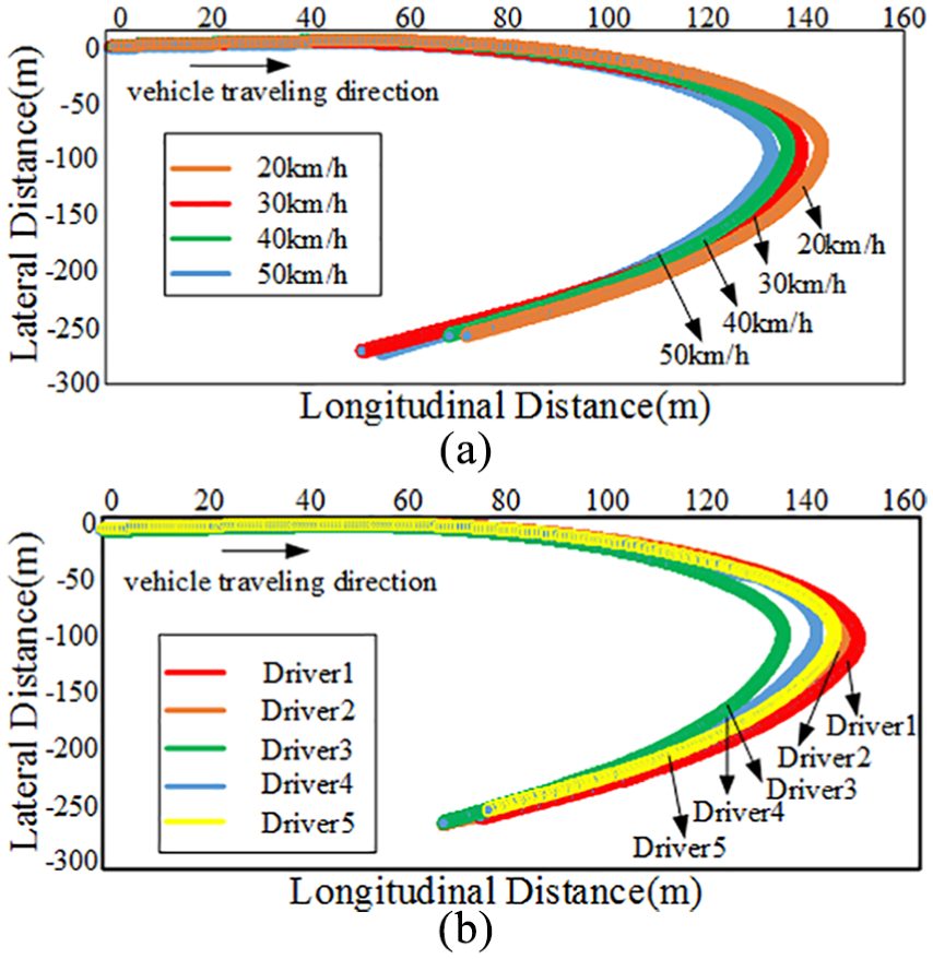
Normal right-steering condition: (a) the effect of different driving speeds on vehicle trajectory and (b) the influence of different drivers on vehicle trajectory.

Figure 1(b) demonstrates the influence of different drivers on vehicle trajectory under the normal right-steering condition. Under the same speed, the driving trajectory of driver 1 is closer to the outside lane. There is a higher possibility of cars crashing ones in the opposite direction. As a result, the driver 1 has a relatively radical driving style. It can also be concluded that the driver 3 has a relatively moderate driving style and the other three drivers have a usual driving style which is neither radical nor moderate. Factors that also affect the driving trajectory under the normal right-steering condition should also include road curvature and preview distance. These two influencing factors are apparent with no need to be analyzed here.

Figure 2(a) shows the effect of different driving speeds on vehicle trajectory under the U-turn condition. It can be seen that at a relatively low speed (10 km/h), skilled drivers tend to turn around at a slower corner speed at the beginning. As a result, the curve that starts the U-turn phase has a longer arc length and is closer to the outside of the road. In this way, the comfort of the passengers can be improved. Because the vehicle speed is slow, at the end of the U-turn, it is easier to control the steering of the vehicle. Therefore, when the vehicle completes the U-turn, the vehicle’s trajectory is closer to the inside of the road. What is contrary is that, when the vehicle speed is high (30 km/h), skilled drivers will increase the steering wheel angle when starting the U-turn operation, thus bringing the vehicle closer to the inside of the road. When the vehicle is completely turned over, the vehicle’s trajectory is closer to the outside of the road. Since normal drivers will try to reduce the speed when U-turning, this article only selects two speeds of 10 and 30 km/h for testing. When the higher speed is chosen in the experiment, it does not match with the actual situation.

Figure 2.

U-turn condition: (a) the effect of different driving speeds on vehicle trajectory and (b) the influence of different drivers on vehicle trajectory.

Figure 2(b) demonstrates the influence of different drivers on vehicle trajectory under the U-turn condition. At the same speed, it can be seen that the driving trajectory of the driver 1 is closer to the inside of the road which is more dangerous because there is a higher possibility of crashing near the edge of the lane. Therefore, it can be concluded again that the driver 1 had a relatively aggressive driving style, which is consistent with the conclusions drawn from the ordinary right-steering condition as mentioned above. The driving trajectory of the driver 3 is opposite to that of the driver 1, and it is closer to the outside of the road. Therefore, it is concluded again that the driver 3 has a relatively stable driving style. The other three drivers from the driving trajectory may not agree with the conclusions drawn from the normal right-steering condition. However, as for the overall trend, the three drivers still have the normal driving style, neither radical nor steady. Factors that also affect the driving trajectory under the U-turn condition should also include the lateral distance (the distance of the vehicle from the left road edge when the vehicle starts to turn around) and the preview distance. These two influencing factors are apparent with no need to be analyzed here.

Under the lane-keeping condition, the speed, driving style, and preview distance are the main factors that affect the driving trajectory. Under the lane-changing condition, apart from the speed, driving style, and preview distance, when the vehicle starts to change lanes, the lateral distance of the vehicle center from the lane line is also a factor of influencing the trajectory.

Vehicle trajectory fitting based on GRNN network

When driving a vehicle, a skilled driver will choose an optimal driving trajectory based on the vehicle and environmental information and then operate the steering wheel, accelerator pedal or brake pedal to make the vehicle run smoothly along the planned path. Although autonomous vehicles can use some advanced algorithms (such as Bezier curves and splines) for path planning based on relevant information, the path that is generated is very different from the actual path taken by the driver, which makes the comfortableness of automatic driving deteriorate. By learning the driving trajectory of skilled drivers under different conditions, the unmanned vehicle can run as smoothly as a car driven by a skilled driver.

Dr DF Specht ²² proposed GRNN in 1991; it is another variation of radial basis neural network.

Suppose x, y are two random variables whose joint probability density is f(x, y). If the observed value of x is known to be x₀, the regression of y with respect to x is

$$E〈y|x_0〉=y\left(x_0\right)=\frac{{\int }_{-\infty }^0\mathrm{yf}(x_0,y)\mathrm{dy}}{{\int }_{-\infty }^{0}f(x_0,y)\mathrm{dy}}$$

(1)

y(x₀) is the predicted value of y under the condition that the input is x₀. Using the Parzen nonparametric estimation, the density function f(x₀, y) can be estimated from the sample data set $\{x_i,y_i{\}}_{i=1}^n$ as follows

$$f(x_0,y)=\frac{1}{n{\left(2\pi \right)}^{\frac{p+1}{2}}{\sigma }^{p+1}}\sum _{i=1}^n{e}^{-d(x_0,x_i)}{e}^{-d(y_0,y_i)}$$

(2)

$$d(x_0,x_i)=\sum _{j=1}^p{[(x_{0j}-x_{\mathrm{ij}})/\sigma ]}^2,d(y,y_i)={[y-y_i]}^2$$

where n is the sample size and p is the dimension of the random variable x.

Substituting equation (1) into equation (2) and exchanging the order of integration and summation, there are

$$y\left(x_0\right)=\frac{\sum _{i=1}^n\left(e^{-d(x_0,x_i)}{\int }_{-\infty }^{+\infty }y{e}^{-d(y_0,y_i)}\mathrm{dy}\right)}{\sum _{i=1}^n\left(e^{-d(x_0,x_i)}{\int }_{-\infty }^{+\infty }{e}^{-d(y_0,y_i)}\mathrm{dy}\right)}$$

(3)

Because ${\int }_{-\infty }^{+\infty }x{e}^{-x^2}\mathrm{dx}=0$ by simplifying the above formula to obtain

$$y\left(x_0\right)=\frac{\sum _{i=1}^{n}y{e}^{-d(y_0,y_i)}}{\sum _{i=1}^n{e}^{-d(y_0,y_i)}}$$

(4)

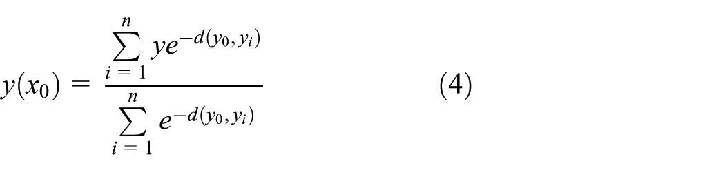
where the numerator is the weighted sum of the y_i values calculated for all training samples.

The GRNN consists of four layers, which are the input layer, the hidden layer, the additive layer, and the output layer, as shown in Figure 3. This article fits the driving trajectory under different conditions through the GRNN network.

Figure 3.

GRNN network structure.

The analysis in the section “Skilled driver steering characteristics analysis” shows the main influencing factors of the vehicle trajectory under normal right-steering, U-turn, lane-keeping, and lane-changing four conditions. The driver 4 was selected to fit the GRNN models because his driving style is closer to the general public’s driving style than the other four drivers. In the GRNN, the longitudinal distance in the two-dimensional plane coordinates in the geographic coordinate system, the driver type, steering condition, and vehicle speed are used as input quantities, and the lateral distance in the two-dimensional plane coordinates in the geographic coordinate system is output.

The fitted trajectory and the actual trajectory of the skilled driver under the four conditions are respectively shown in Figures 4(a), 5(a), 6(a), and 7(a). It can be seen from the figure that the obtained trajectory is consistent with the actual trajectory of the test and can reflect the characteristics of the driving trajectory selected by the skilled driver under the same condition. Figures 4(b), 5(b), 6(b), and 7(b) reveal respectively the lateral deviations between the fitted trajectory and the actual trajectory of the skilled driver under four conditions. It can be seen from Figures 4(b) and 5(b) that the lateral deviation of the turning point is relatively large under the normal right-steering condition and the U-turn condition because the road curvature is small and the trajectory is complicated during the turning process. According to the simulation statistics, the maximum lateral deviation is 0.34 and 0.35 m, respectively. Under the conditions of lane-keeping and lane-changing, it can be seen from Figures 6(b) and 7(b) that the driving trajectory of the vehicle is relatively simple, so the fitting is better, and the lateral deviation is smaller. According to the simulation statistics, the maximum lateral deviation is respectively 0.035 and 0.11 m.

Figure 4.

Normal right-steering condition: (a) trajectory fitting and (b) lateral deviation.

Figure 5.

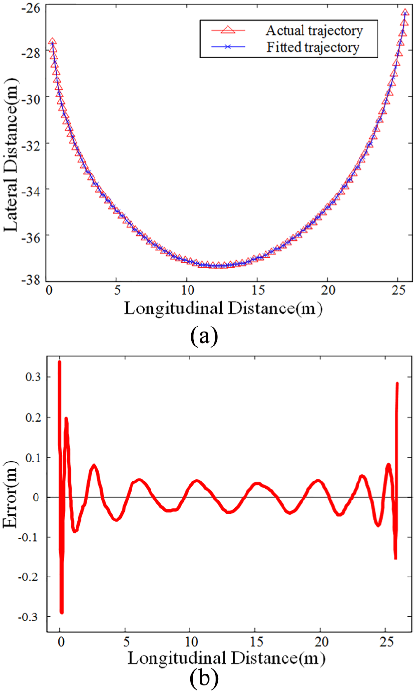
U-turn condition: (a) trajectory fitting and (b) lateral deviation.

Figure 6.

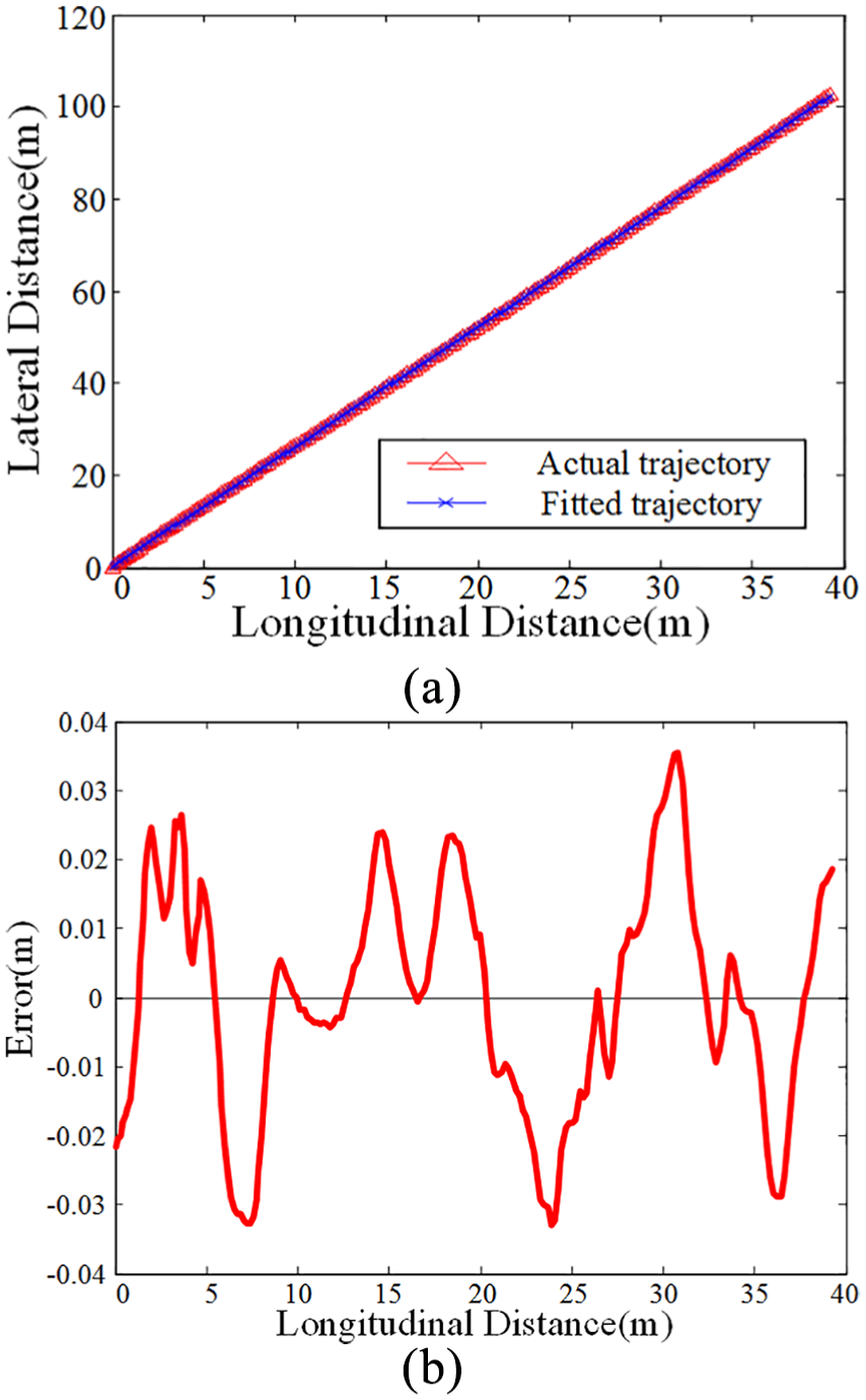
Lane-keeping condition: (a) trajectory fitting and (b) lateral deviation.

Figure 7.

Lane-changing condition: (a) trajectory fitting and (b) lateral deviation.

Driver modeling process based on MPC

Driver model based on model prediction

Typically, based on some theories,^23–25 the driver model includes a systematic input controller, enabling the intelligent vehicle to run at the expected rate along the expected trajectory.

In the two-dimensional plane coordinates of the geographic coordinate system, the vehicle must start from a fixed initial point, and a series of discrete trajectory points can be used to form the expected trajectory of the intelligent vehicle at any time (t). The expected trajectory refers to a geometric curve $f(x_r(t))$ . The expected trajectory applied in this section is based on the nonlinear fitting made by GRNN network about the skilled driver’s real vehicle trajectory. At the same time, the speed that is given refers to the speed variable in the general aspect, which is also known as the reference control input. Physical quantities such as yaw rate and front wheel angle are controlled for their input.

The following hypotheses are made for the driver model established in this article. First, the reference trajectory of vehicle, road conditions, and road adherence index are known. Second, vehicle location, interior conditions as well as signals such as lateral speed, accelerated speed, and wheel speed are known.

The driver model is established based on all known parameters of environment and interior vehicle conditions. According to the hypotheses mentioned above, the principle of the driver model tracking trajectory process is shown in Figure 8, and the driver model based on MPC is presented in Figure 9.

Figure 8.

Driver model tracking trajectory process.

Figure 9.

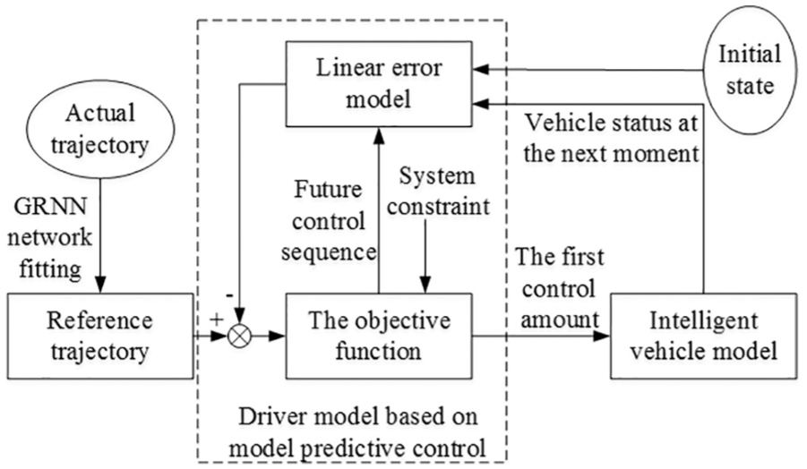
Driver model based on MPC.

Vehicle kinematics model

In order to guarantee the safety and comfortableness, adept drivers tend to decrease the speed without exception consciously. Vehicles in both reality and test run at a slow rate under different steering conditions. Therefore, to make the calculation more convenient, this part mainly establishes vehicle kinematics model.

In the ground fixed coordinate system OXY, vehicle kinematics equation

$$\left[\begin{array}{c}\stackrel{·}{x}\hfill \\ \multicolumn{1}{c}{\stackrel{·}{y}}\\ \multicolumn{1}{c}{\stackrel{·}{\phi }}\end{array}\right]=\left[\begin{array}{c}\cos \phi \hfill \\ \multicolumn{1}{c}{\sin \phi }\\ \multicolumn{1}{c}{\tan \phi /l}\end{array}\right]v$$

(5)

where $(x,y)$ is the coordinates of the center point of the rear axle of the wheel, $\phi$ is the heading angle of the vehicle body, $\delta$ is the front wheel angle, v is the rear axle speed of the vehicle, and l is the wheelbase.

From equation (5), the system can be seen as a control system with inputs $u(v,\delta )$ and state variables $\xi (x,y,\phi )$ . Its general form is

$$\stackrel{·}{\xi }=f(\xi ,u)$$

(6)

The kinematic model of the above vehicle can be used to describe a given reference trajectory. The “r” is used to represent the reference amount. The general form is

$${\stackrel{·}{\xi }}_r=f({\xi }_r,u_r)$$

(7)

where ${\xi }_r=[\begin{array}{ccc}{x}_r\hfill & y_r\hfill & {\phi }_r\hfill \end{array}{]}^T$ , $u_r=[v_r,{\delta }_r]$ .

Equation (7) is a first-order Taylor series expansion at the reference trajectory point to obtain

$$\begin{array}{c}\stackrel{·}{\xi }=f({\xi }_r,u_r)\hfill \\ +{\frac{\partial f(\xi ,u)}{\partial \xi }|}_{\xi ={\xi }_r,u=u_r}(\xi -{\xi }_r)+{\frac{\partial f(\xi ,u)}{\partial u}|}_{\xi ={\xi }_r,u=u_r}(u-u_r)\hfill \end{array}$$

(8)

Subtracting equation (7) from equation (8) yields

$$\begin{array}{c}\multicolumn{1}{c}{\stackrel{·}{\stackrel{~}{\xi }}=\left[\begin{array}{c}\stackrel{·}{x}-{\stackrel{·}{x}}_r\hfill \\ \multicolumn{1}{c}{\stackrel{·}{y}-{\stackrel{·}{y}}_r}\\ \multicolumn{1}{c}{\stackrel{·}{\phi }-{\stackrel{·}{\phi }}_r}\end{array}\right]=\left[\begin{array}{ccc}0\hfill & 0\hfill & -v_r\sin {\phi }_r\hfill \\ \multicolumn{1}{c}{0}& 0\hfill & v_r\cos {\phi }_r\hfill \\ \multicolumn{1}{c}{0}& 0\hfill & 0\hfill \end{array}\right]\left[\begin{array}{c}x-x_r\hfill \\ \multicolumn{1}{c}{y-y_r}\\ \multicolumn{1}{c}{\phi -{\phi }_r}\end{array}\right]+B_{k,t}}\\ =\left[\begin{array}{cc}\cos {\phi }_{r}T\hfill & 0\hfill \\ \multicolumn{1}{c}{\sin {\phi }_{r}T}& 0\hfill \\ \multicolumn{1}{c}{\tan {\delta }_r/l}& v_r/l{\cos }^2{\delta }_r\hfill \end{array}\right]\left[\begin{array}{c}v-v_r\hfill \\ \multicolumn{1}{c}{\delta -{\delta }_r}\end{array}\right]\hfill \end{array}$$

(9)

The above formula is the linear error model required for the path tracking of the driver model after linearization. In order to facilitate the design of the predictive model controller, the discretization of equation (9) is performed

$$\tilde{\xi }(k+1)=A_{k,t}\tilde{\xi }\left(k\right)+B_{k,t}\tilde{u}\left(k\right)$$

(10)

where

$$A_{k,t}=\left[\begin{array}{ccc}1\hfill & 0\hfill & -v_r\sin {\phi }_{r}T\hfill \\ \multicolumn{1}{c}{0}& 1\hfill & v_r\cos {\phi }_{r}T\hfill \\ \multicolumn{1}{c}{0}& 0\hfill & 1\hfill \end{array}\right]$$

$$B_{k,t}=\left[\begin{array}{cc}\cos {\phi }_{r}T\hfill & 0\hfill \\ \multicolumn{1}{c}{\sin {\phi }_{r}T}& 0\hfill \\ \multicolumn{1}{c}{\tan {\delta }_{r}T/l}& v_{r}T/l{\cos }^2{\delta }_r\hfill \end{array}\right]$$

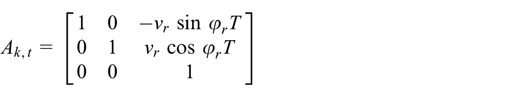
T is the sampling time.

The objective function of the driver model

The objective function design of the driver model should aim to enable the vehicles to respond rapidly and the expected trajectory to tracked smoothly. The paper adopts the method of state deviation of the controlling system and optimizing controlling factors to design trajectory following controller. The objective function of the design is as follows

$$\begin{array}{c}J\left(k\right)=\hfill \\ \sum _{j=1}^N{\tilde{\xi }}^T\left(k+j|k\right)M\tilde{\xi }(k+j)+{\tilde{u}}^T(k+j-1)N\tilde{u}(k+j-1)\hfill \end{array}$$

(11)

where M and N are weight matrices.

The first and second factors respectively stand for the ability of system following reference trajectory and the constraint of variable changes. Although the designed objective function can be presented in the form of standard quadratic programming, controlled variables during each sampling period cannot be restricted, and it is difficult to secure the consistency of controlling variables. As a result, the above-mentioned objective function can converse as follows ²⁶

$$\begin{array}{c}J\left(k\right)=\sum _{i=1}^{T_p}\Vert y\left(k+i|t\right)-y_{\mathrm{ref}}\left(k+i|t\right){\Vert }_M^2\hfill \\ +\sum _{i=1}^{T_c-1}\Vert \mathrm{\Delta }U\left(k+i|t\right){\Vert }_N^2+\eta \sum _{i=1}^{T_p}{s}_{\mathrm{opt}}^2\hfill \end{array}$$

(12)

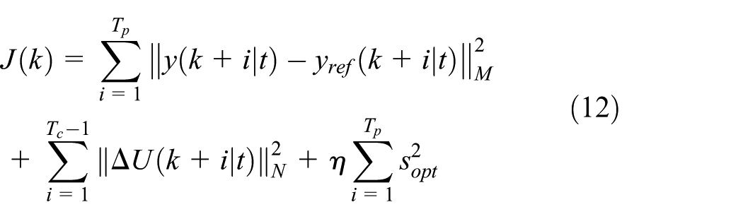
where T_p is the prediction time domain (T_p = 60), T_c is the control time domain (T_c = 30), η is the relaxation coefficient (η = 10), and S_opt is the relaxation variable.

The objective function after the conversion is characterized in that the control increments together with the slack variables can not only directly limit the control increments, but also obtain a feasible solution during the running process. In the designed objective function (12), it is necessary to predict and calculate the system output in the next period.

The constraints of the driver model

The control quantity limit constraint and the incremental control constraint are the main constraint forms considered in this article. The expressed form of the control quantity is as follows

$$u_{min}(t+k)\le u(t+k)\le u_{max}(t+k),k=0,1,\dots ,T_c-1$$

(13)

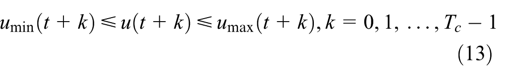
The control incremental constraint expression is

$$\begin{array}{c}\mathrm{\Delta }{u}_{min}(t+k)\le \mathrm{\Delta }u(t+k)\hfill \\ \le \mathrm{\Delta }{u}_{max}(t+k),k=0,1,\dots ,T_c-1\hfill \end{array}$$

(14)

After transforming the designed objective function into a standard quadratic form, the following optimization problems are calculated under constraints

$$\begin{array}{c}J(\psi \left(t\right),u(t-1),\mathrm{\Delta }U\left(t\right))\hfill \\ ={[\mathrm{\Delta }U{\left(t\right)}^T,s_{\mathrm{opt}}]}^T{H}_t[\mathrm{\Delta }U{\left(t\right)}^T,s_{\mathrm{opt}}]\hfill \\ +G_t[\mathrm{\Delta }U{\left(t\right)}^T,s_{\mathrm{opt}}]\hfill \end{array}$$

(15)

$$s.t.\{\begin{array}{c}\mathrm{\Delta }{U}_{min}\le \mathrm{\Delta }{U}_t\le \mathrm{\Delta }{U}_{max}\hfill \\ \multicolumn{1}{c}{U_{min}\le A\mathrm{\Delta }{U}_t+U_t\le U_{max}}\end{array}$$

(16)

where

$$H_t=\left[\begin{array}{cc}{\Theta }_t^{T}M{\Theta }_t+N\hfill & 0\hfill \\ \multicolumn{1}{c}{0}& \eta \hfill \end{array}\right]$$

$$G_t=\left[\begin{array}{cc}2e_t^{T}M{\Theta }_t\hfill & 0\hfill \end{array}\right]$$

$e_t$ is the tracking error in the predict time domain.

Solving equation (15) throughout the control process, control inputs incremental set in the control time domain is obtained

$$\mathrm{\Delta }{U}_t^{*}={[\mathrm{\Delta }{u}_t^{*},\mathrm{\Delta }{u}_{t+1}^{*},\dots ,\mathrm{\Delta }{u}_{t+T_c-1}^{*}]}^T$$

(17)

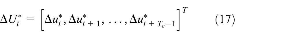
The first element in the control sequence is applied to the system as an actual control input increment, resulting in

$$u\left(t\right)=u(t-1)+\mathrm{\Delta }{u}_t^{*}$$

(18)

After entering the next control cycle, the above process is repeated, and path tracking of the reference trajectory by the driver model can be realized by such a cycle.

Simulation analysis of driver model under different conditions

In order to verify the validity of the driver model based on MPC in this article established, the normal right/left-steering, U-turn, lane-keeping, and lane-changing four conditions are simulating under different vehicle speeds, and this article is analyzing and discussing from the two aspects of path trajectory and lateral deviation. The vehicle model parameters are shown in Table 3.

Table 3.

Vehicle model parameters.

Parameter name	Numerical value	Unit
Vehicle quality	1558	kg
Length/width/high	4915/1845/1470	mm
Wheelbase	2775	mm
Front wheel distance/rear wheel distance	1585/1580	mm
The distance from the vehicle centroid to the front and rear axles	1110/1665	mm
Moment of inertia of the vehicle around the X-, Y-, Z-axis	671.3/1972.8/2315.3	kg m2
Tire specifications	225/50 R17

In order to facilitate the comparative analysis, a driver model based on the single-point preview and a path tracking algorithm based on the β-spline curve are designed and compared with the driver model and algorithm proposed in this article. The reason for choosing a driver model based on single-point preview is that the algorithm has a representative in the driver model based on the “preview-follow” theory. ²⁷ The β-spline curves are reference trajectories that need to be tracked, and the tracking algorithm uses tracking based on a purely tracking algorithm based on geometric principles. The purpose of selecting a path tracking algorithm based on the β-spline curve is that the algorithm represents a method of tracking the target path by fitting a smooth geometric curve, such as β-spline curve,^28,29 and Bezier curve.^30,31 Gomez-Bravo et al. ²⁸ propose continuous curvature path generation based on the β-spline curve for parking maneuvers.

It can be seen from Figure 10 that under the normal right-steering condition, at the same vehicle speed, the model predictive driver model proposed in this article considering the steering characteristics of the skilled driver can well track the reference path for steering operation. The driver model based on single-point preview and the tracking algorithm based on the β-spline curve also track the reference path. However, it can be seen from the two aspects of the vehicle trajectory and the lateral deviation that the tracking effect of the two is poor compared with the model based on predicative model control. Among them, the tracking algorithm based on β-spline curve shows apparent deviation at the initial stage of simulation and when the steering angle is large. This is because the algorithm does not consider the motion or dynamic model of the vehicle system, and its tracking path is composed of a group of smooth parametric curve segments which are approximated by a polygon. As the vehicle speed increases, the lateral deviation will increase accordingly. However, due to the lower speed of the simulated setting, the degree of lateral deviation increasing is not obvious. This is because the steering speed is set at a low rate according to the habit of skilled drivers driving slowly when turning around. As a result, the simulation results of vehicles turning around at a significant speed are not given.

Figure 10.

Simulation results of vehicle trajectory and lateral deviation under the normal right-steering condition: (a) vehicle speed of 20 km/h, (b) vehicle speed of 35 km/h, and (c) vehicle speed of 50 km/h.

It can be seen from Figure 11 that under the U-turn condition, at the same vehicle speed, it can also be obtained that the driver model based on MPC has better path tracking effect than the single-point preview driver model and the tracking algorithm based on the β-spline curve. Meanwhile, because the U-turn condition is more complicated than the ordinary right-steering condition, the driver model based on the MPC has a sizable lateral deviation.

Figure 11.

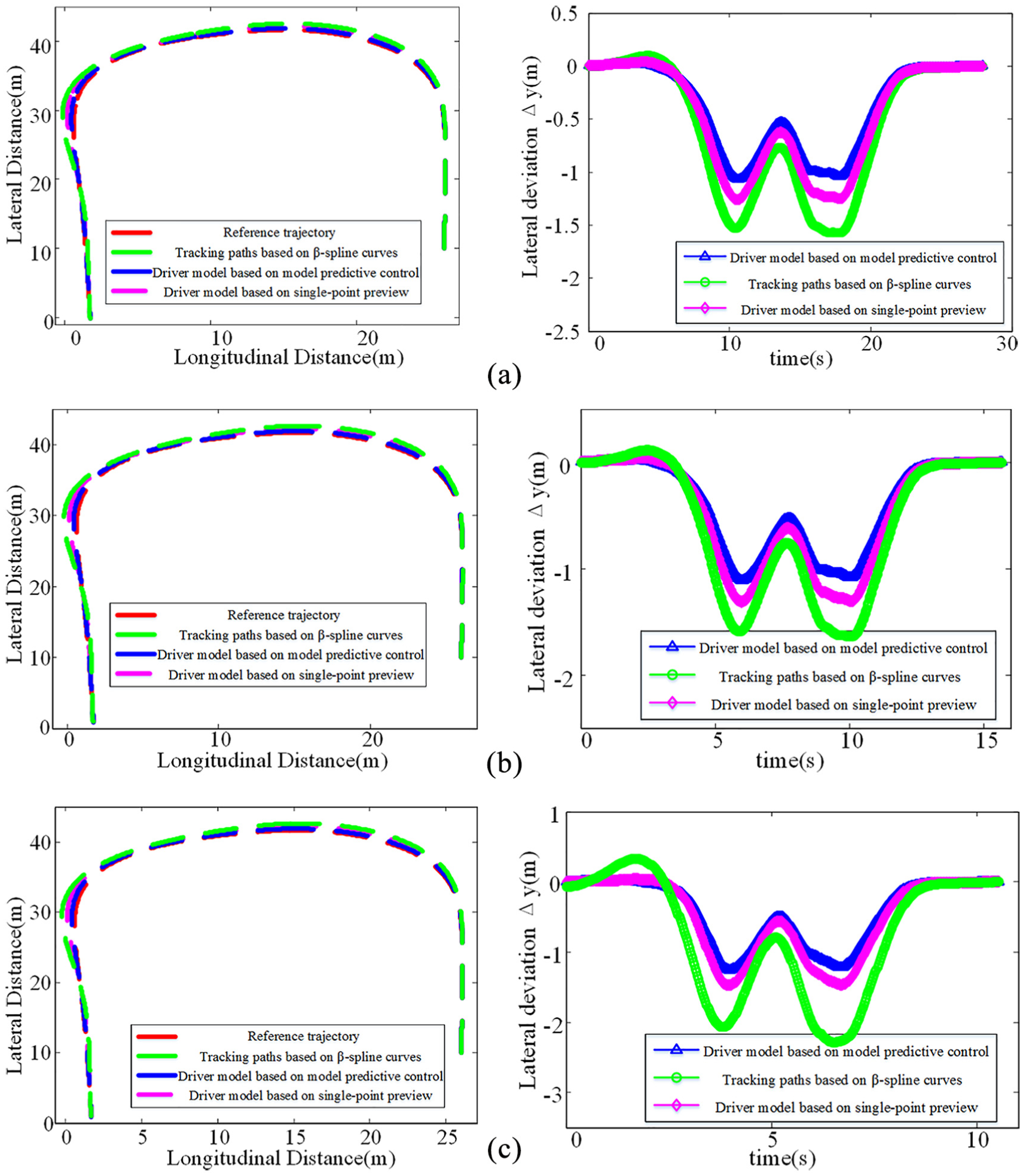
Simulation results of vehicle trajectory and lateral deviation under U-turn condition: (a) vehicle speed of 10 km/h, (b) vehicle speed of 20 km/h, and (c) vehicle speed of 30 km/h.

As can be seen from Figures 12 and 13, under the lane-keeping condition and lane-changing condition, at the same vehicle speed, it can also be obtained that the driver model based on MPC has better path tracking effect than the single-point preview driver model and the tracking algorithm based on the β-spline curve. Meanwhile, since the two conditions are more straightforward than the normal right-steering condition, the driver model based on the MPC has a small lateral deviation.

Figure 12.

Simulation results of vehicle trajectory and lateral deviation under the lane-keeping condition: (a) vehicle speed of 30 km/h, (b) vehicle speed of 35 km/h, and (c) vehicle speed of 40 km/h.

Figure 13.

Simulation results of vehicle trajectory and lateral deviation under the lane-changing condition: (a) vehicle speed of 30 km/h, (b) vehicle speed of 35 km/h, and (c) vehicle speed of 40 km/h.

Conclusion

Based on the nonlinear fitting results of GRNN on the real trajectory of skilled drivers, this article establishes a predictive driver model with the steering characteristics of skilled drivers into consideration. Simulation analysis is performed, and it is compared with the traditional single-point preview driver model and based on the path tracking method based on the β-spline curve. The results show that the model predictive driver model considering the steering characteristics of the skilled driver can better track the vehicle reference trajectory, and the following effect is better than that of the two traditional methods.