Sage Journals: Discover world-class research

Abstract

Taking the test signals of magneto-rheological vibration system under different states as research objects, four Generalized Regression Neural Network (GRNN) prediction algorithms, based on time series, time series Auto-Regressive (AR) model coefficients, time series box dimensions, and Variational Modal Decomposition (VMD) box dimensions, are designed. Moreover, four Back Propagation Neural Network (BPNN)comparative prediction algorithms, based on the four previous parameters, are also designed. These eight algorithms are applied to predict vibration damping efficiency of the system. The prediction results show that, compared to the BPNN prediction algorithm, the corresponding four GRNN prediction algorithms have the advantages of strong self-learning ability, fast convergence speed, high prediction accuracy, and stable prediction results. Among the eight prediction algorithms, the GRNN prediction algorithm, based on VMD box dimension, forecasts the results with good stability, better self-learning ability, and higher computing speed, which can maximize the prediction accuracy of the system, the minimum prediction error can reach 1.9049% when the parameters K = 4, N = 33, and Spread = 0.601. To sum up, through parameter optimization, the optimal parameter combination scheme of GRNN prediction algorithm, based on VMD box dimension, is obtained, and the best prediction effect is achieved.

Keywords

Fractal dimension variational modal decomposition generalized regression neural network

Introduction

Magneto-Rheological (MR) vibration system is a multi-input complex system, mainly used in automotive, transportation, construction engineering, mechanical engineering, and other engineering domains. In order to obtain different damping effects, the system usually changes its damping performance by controlling different input currents.^1,2 Chen et al.³ established multiple dynamic models of the vibration system, compared and analyzed different modeling accuracies, and calculated the dynamic characteristic parameters of the system through the relationship between the coefficients of the time series and its Auto-Regressive (AR) model. In addition, they analyzed the performance changes of the vibration damping system under different states. Chen et al.⁴ calculated the correlation between the time series correlation dimension, the box dimensions and the dynamic performance parameters of the vibration damping system, they found that the change of fractal dimension reflects the change of dynamic performance of vibration system to a certain extent; thus, this variation was considered as a parameter to measure the complexity of the system signal. For the state of the MR vibration system, the calculation of prediction is large and the efficiency is low, when the detected time series are directly used as the eigenvector to predict the state. It is necessary to find parameters or vector dimensionality reduction suitable for reflecting the characteristics of the system to improve the prediction efficiency and meet the high prediction accuracy. Meanwhile, the number of state samples of the system is small. Traditional prediction methods, the prediction results are more sensitive to changes in the number of training samples, and the prediction effect is poor in the small sample prediction, and it is difficult to obtain high prediction accuracy. A complicated system signal can be broken down into numerous modal components by Variational Modal Decomposition (VMD),⁵ each of which has a particular frequency and signal properties. VMD has been also applied to signal noise reduction, fault diagnosis, state recognition, feature extraction, and other research in recent years. As for the Back Propagation Neural Network (BPNN)⁶ and the Generalized Regression Neural Networks (GRNN), they are widely used in condition prediction, classification, and troubleshooting. The combined application of VMD, GRNN, and fractal dimension is still relatively small, and there has been no comprehensive application in the state prediction of MR vibration reduction systems.⁷

In this paper, the main objective consists of taking the MR vibration system as the research object and collecting the time series of the vibration signal in different states of the system, after establishing four feature vector extraction methods, such as time series, AR model coefficient of time series, box dimension of time series, box dimension of VMD component, etc. Then, using two prediction models, that is, BPNN and GRNN, eight state prediction algorithms are determined to predict the vibration damping efficiency of the state. Thus, the characteristic parameter extraction method, in addition to the best predictive model and its parameters, which are most suitable for the vibration signal of the system, are studied and determined from the comparative analysis.

Thus, this paper will be divided as follow: in section 2, the basic theory of the prediction methods will be presented whereas the experimental data will be provided in section 3. Section 4 will introduce the eight predictive algorithms and the results will be displayed in section 5. Finally, section 6 will conclude this work and show some future ideas that may enhance this research.

Basic theory

Time series box dimension

Box dimension is the main parameter of fractal theory. Box dimension of time series reflects the complexity of time series signal and measures the irregularity of the signal.^8,9 Suppose x is a closed set on n-dimensional Euclidean space (Rⁿ), for time series, when $x (i) \subset X$ , and if Rⁿ is divided into meshes whose width is △ whenever possible, and $N_{Δ}$ is the grid count of the set X, the box dimension is defined as^4,10,11:

d = lim_{Δ \to 0} (- \lg N_{Δ} / \lg Δ)

(1)

VMD

VMD is an adaptive, completely non-recursive method of modal variation, and signal processing. The method can adaptively obtain matching modal components according to the number of modal decomposition¹² which can improve the stationarity of complex and nonlinear time series to obtain a relatively stationary sub-sequence containing multiple different frequency scales. The method is suitable for non-stationary time series while the core problem is to determine the number of decomposition modes (K) and the quadratic penalty factor (M).¹³

BPNN and GRNN

BPNN includes the input layer, the implicit layer and the output layer and it is considered a kind of supervised learning.¹⁴ Many parameters affect BPNN, where the most important are the weight, the threshold, and the number of hidden layers. As for GRNN, it includes four layers (input, pattern, summation, and output). It is a common intelligent neural network budget and classification algorithm, which is an unsupervised network model where generally only one Spread parameter, which is distribution density of radial basis function, needs to be determined. Concerning GRNN, the parameters’ adjustment is convenient, its calculation convergence speed is fast, and its prediction accuracy is high. Thus, GRNN is more suitable for prediction when being applied for small samples.¹⁵

Experimental data sources

This experimental data comes from Huang et al. self-made MR shock absorber and test system (as shown in Figure 1). The system takes the MR shock absorber as the control object and changes its performance by adding input current. So, the data collection of this experiment in the control current I = 0,0.5,1,1.5,2,2.5A, taking into account the operating frequency range of the system and the entire vibration damping system at the operating frequency f = 20, 25, 30, 35, 40, 45, and 50 Hz. The sampling frequency is 500 Hz according to Nyquist Sampling theory, thus constituted 42 working states. The displacement, in addition to the acceleration signal and the vibration damping efficiency, are collected separately in different operating state.^1,2

Figure 1.

Schematic diagram of the vibration system.

Design of predictive algorithms and comparative experiments

Eight prediction algorithms are established for the state prediction by designing four feature parameter extraction methods and selecting the BPNN and the GRNN models. Through the comparative evaluation of prediction effect, the prediction algorithm suitable for the system is determined, and the optimal combination scheme of parameters, involved in the algorithm, is considered. Samples reconstructed by the characteristic parameters of the 42 signals and their corresponding vibration damping efficiency are divided into a training set and a test set. In order to compare the influence of different feature parameter extraction methods on the test effect, and to evaluate the self-learning ability of the network, a fixed test set of six samples is used, and the number of training sets (N) increases from 7 to 36. Moreover, the influence of the training set changes on the prediction results, under different feature parameter extraction methods, is investigated.

Two models of BPNN and GRNN are selected for prediction and comparative analysis. The minimum prediction variance is used as the parameter optimization goal, and the test average error percentage (absolute value) R of the six test samples is applied as a parameter for evaluating the prediction effect. The effect parameter equation is listed as follows:

R = \frac{1}{6} \sum_{i = 1}^{6} | (t_o u t p u t_{i} - t_i n p u t_{i}) * 100 % / t_i n p u t_{i} |

(2)

where $t_outpu t_{i}$ represents the predicted value of the vibration damping efficiency, and $t_inpu t_{i}$ . indicates the experimental measurement of the vibration damping efficiency.

In order to reduce the uncertainty of BPNN prediction value, forecasts are repeated for five times, then the average test error percentage (absolute value) $R_{j}$ (j = 1,2,3,4,5) of the six test samples, obtained at the optimal number of layers, is calculated. Finally, the average $\bar{R}$ of five predictions is taken, and the $\bar{R} - N$ curves are plotted.

\bar{R} = \sum_{j = 1}^{5} R_{j}

(3)

GRNN prediction algorithm based on time series

The flowchart of GRNN prediction algorithm, based on time series, is shown in Figure 2(a), and the main steps are listed below:

(1) Pre-processing of vibration signals, the time series (y_i) is extracted for analysis;

(2) 42 states of time series y_i are taken as the characteristic vector, these characteristic vector and the damping efficiency corresponding to the state constitute 42 samples;

(3) The last six test samples are taken as the test set, the number of training sample sets (N) changed from 7 to 36 to form different combination sample sets;

(4) Different Spread values are set at certain intervals, and the GRNN model is applied to train and test different combined sample sets, and the best Spread value and corresponding test average error (absolute value) R, under each combined sample set, are determined by the minimum variance between the predicted value and the experimental value.

Figure 2.

Flowchart of four GRNN prediction algorithms. (a) GRNN algorithm based on time series, AR coefficient, time series box dimension and (b) VMD-box dimension-GRNN algorithm.

GRNN prediction algorithm based on AR model coefficients of time series

Compared to GRNN prediction algorithm based on the time series, the main difference of GRNN prediction algorithm based on time series AR model coefficients is the time series AR model coefficients, which were extracted as eigenvector in step (2), keeping the other steps without changes. The flowchart of this algorithm is shown in Figure 2(a).

GRNN prediction algorithm based on time series box dimension

GRNN prediction algorithm based on time series box dimension differs from the above two prediction algorithms in step (2) where the time series dimension (as eigenvector) are extracted, and the other steps are the same. Its flowchart is shown in Figure 2(a).

VMD-GRNN prediction algorithm based on time series box dimension

The prediction algorithm flow is shown in Figure 2(b), and the main steps to implement it are as follows:

(1) Preprocess the vibration signal and extract the analyzed time series y_i;

(2) Given the secondary penalty factor M₀, set the modes number (K = 1,2,3,……,10) of VMD;

(3) VMD is carried out under different K values, and the 42 states’ corresponding decomposed modal components are generated;

(4) Box dimension (D_i, i = 1∼K) of K modal components in the 42 states are calculated with respect to the box dimension and the damping efficiency;

(5) Taking the last six test samples as the test set, the number of training sample sets N varies from 7 to 36 to form different combination sample sets;

(6) Set the different Spread values at certain intervals, then apply GRNN model to train and test different combined sample sets and determine the best Spread and its corresponding test average error (absolute value) R under each sample set combination along with the minimum variance between the predicted value and the experimental value;

(7) Draw R-N curves corresponding to different K values, then compare and determine the optimal K;

(8) Set different secondary penalty factor (M) at certain intervals under the optimal K, re-perform K modal decomposition, then repeat steps (4)−(6);

(9) Compare the R value under different M values, and determine the best M value when the minimum R value is selected.

Four prediction algorithms of the BPNN model are developed to compare the differences in prediction effects and identify the optimal parameters in order to compare the impacts of the various prediction algorithms mentioned above. The number of hidden layers has a greater impact on the prediction accuracy for four prediction algorithms of BPNN model. In order to find the optimal number of hidden layers, using the minimum mean square error, we varied the number of layers (n) between 1 and 30 for prediction calculation and we find the optimal number of hidden layers having the minimum variance. Repeating the calculation five times under each sample set combination when using BPNN prediction, the calculation result takes the average of these five measurements.

Results analysis

Predict results based on time series

Taking the time series directly as a feature vector for training and testing, Figure 3 plots the R-N relationship curves of BPNN and GRNN under different training samples. The average error (absolute value) of the five calculations of six test samples, predict by BPNN model, is mostly more than 10%. The average minimum error of the five predictions is 7.5331%, and the calculation consumes a lot of machine hours, the impact and fluctuation of the sample number change on the test error are larger, especially in the case of a small number of samples (when N is less than 15), the average test error is greater than 20%. When N is greater than 15, the average error of the test is above 10%. The average error of GRNN prediction decreases significantly with the increase of the training sample number and the overall error value is smaller than that of the BPNN model. The error is less than 8% when the training sample exceeds 15 and the minimum average error is 6.12031%. This yields in concluding that, for GRNN, the error data stability is better, the prediction speed is faster, the overall self-learning ability is stronger; thus, GRNN prediction algorithms, based on time series, shows obvious advantages over BPNN prediction algorithms.

Figure 3.

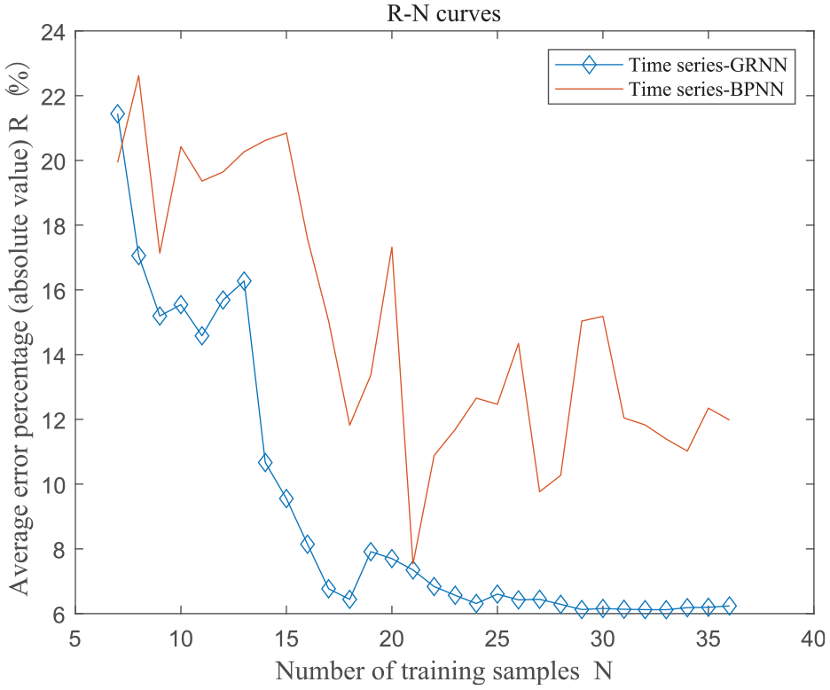
R-N curves based on time series.

Predict results based on coefficients of time series AR model

While time series AR model is established, the coefficients of the AR model under the second order cumulative amount are extracted as state characteristic parameters, and they are used as inputs for BPNN and GRNN model. The vibration damping efficiency is used as the output for training and prediction. The prediction calculation results (shown in Figure 4) show that, under different training sample number N, the average error (absolute value) of the five calculations of the six test samples, predicted by the BPNN model, is mostly above 10%, and the average minimum error is 6.8414%. The change of sample number N has a greater impact on the test error, especially in the case of a small number of samples (when N is less than 15) where the average test error is more than 15%. With the same eigenvector as input, the average error of GRNN prediction of six samples is significantly reduced relative to the BPNN prediction error, and the number of training samples N is relatively stable and equal to 12, and most of the average errors are below 6%. This shows that, using GRNN, the prediction error of time series AR model coefficient is smaller, the stability is better, and the self-learning ability is stronger than that of BPNN, especially when the training set reaches a certain number of samples.

Figure 4.

R-N curves based on AR model coefficients of time series.

Compared to time series direct prediction method, the consumption of AR model coefficient method is significantly reduced, and the prediction accuracy is slightly improved, which is due to the reduction of the characteristic parameters from 500 to 12. This effectively improves the prediction efficiency by reducing dimensionality. Time series AR model coefficients can reflect the characteristics of the system much better, and as a characteristics parameter, it can improve the prediction accuracy of the system to a certain extent while effectively improving efficiency.

Prediction results based on time series box dimensions

Figure 5 presents the relationship curve between the mean error R and the training sample N, calculated by the BPNN and the GRNN algorithms based on time series box dimensions. As can be seen from Figure 5, the mean percentage of the minimum error average, calculated for the BPNN model, is 6.2075%, and the time series box dimension is used as a single input parameter, the average minimum error is varying in the range of 6%–10%. As for the GRNN model, the minimum error average is 4.9251%, the average minimum error is maintained at 5%–9%, and the prediction error of the two models training sample number N is slightly reduced but the change is not large. This demonstrates that, in comparison to direct time series and time series AR model coefficient, time series box dimension taken as a measure of the complexity of time series better reflects the state and characteristics of the system. The prediction accuracy is also improved, the consumption time is minimal, and the prediction effect advantage is clear. A comparison between BPNN and GRNN algorithms, based on the of time series box dimension, yields in confirming that GRNN algorithms has higher prediction accuracy.

Figure 5.

R-N curves based on box dimension of time series.

Prediction results based on time series box dimension of VMD components

For a complex time series signal, under the specific decomposition number K and penalty factor M, the variational modal decomposition can result in K time series components of different frequency components. Figure 6 shows the original displacement signal which is recorded by the MR vibration and testing system at the control current I = 2.5 A, the vibration frequency f = 50 Hz, and its three decomposed components (IMF) by VMD at K = 3 & M = 99, where the IMF1 component is the most energetic low-frequency signal and IMF2 component is close to the resonant signal. With different combinations of K and M, the obtained signal components vary. In this paper, at the given M = 99, 42 state signals are decomposed by VMD according to K = 1,2,3,…,10, and the modal component (IMF_i, i = 1∼K) of the same number of each state is obtained. Box dimension D_k of K components is calculated, then D_k and the vibration damping efficiency form 42 groups of samples, which are predicted according to the “time series-VMD-box dimension-GRNN” prediction algorithm and compared with the prediction results of the “time series-VMD-box dimension-BPNN” prediction algorithm.

Figure 6.

Original signal and its mode components by VMD.

Influence of K on prediction results

Given M = 99, and using the “time series-VMD-box dimension-BPNN” prediction algorithm and “time series-VMD-box dimension- GRNN” prediction algorithm, under different values of K, the prediction average error R and the corresponding data of the training sample number N are plotted as shown in Figures 7 and 8.The minimum average error value R_min of the two algorithms, under different K, is listed in Table 1, and the R_min-K relationship curve is shown in Figure 9.

Figure 7.

R-N curves under time series-VMD-box dimension-BPNN.

Figure 8.

R-N curves under time series-VMD-box dimension-GRNN.

Table 1.

Correspondence between average minimum error and number of decomposition modes.

K of VMD	R _min by BPNN (%)	R _min by GRNN
1	6.3844	6.3234
2	5.9286	6.3320
3	4.6552	3.8660
4	6.4128	2.7905
5	7.1296	4.8825
6	5.5989	4.7648
7	6.5948	4.5726
8	9.2644	6.4395
9	7.7222	4.6599
10	9.9162	6.1281

Figure 9.

R _min -K diagram under two models.

As shown in Figure 9, in addition to VMD(1) (K = 1) under the two algorithms, the prediction error R decreases overall with the increase of the training sample number N. This indicates that increasing the training sample can improve the prediction accuracy, but the corresponding change ratio of the two algorithms is obviously different. The corresponding curve of BPNN prediction algorithm, based on VMD-box dimension, declines slowly, while the corresponding curve of GRNN algorithm, based on VMD-box dimension, drops sharply at the beginning, and the decline rate becomes slower after N gets greater than 10. This indicates that the algorithm converges faster and the self-learning ability is stronger. Comparing the prediction error values of the two algorithms, the VMD-box dimension-GRNN curve is smoother, and the VMD-box dimension-BPNN prediction error value fluctuates greatly, which is mainly caused by the uncertainty characteristics of the BPNN. Most of the VMD-box-GRNN prediction error are below 7%, which is significantly lower than VMD-box dimension-BPNN prediction.

At K = 1, R-N curves for both algorithms are close to the horizontal position, which indicates that the training sample number N has little effect on the prediction results, and VMD(1) (K = 1) has a large advantage in the case of a small samples number, which is more suitable for the prediction application of a small samples number. Compared to the prediction based on time series box dimension, the prediction accuracy is relatively close, but the prediction error after VMD(1) is more stable with the change of sample number, which is due to the effect of noise reduction after VMD.

Table 1 and Figure 9 show that R_min, varies under different values of K by two models.When K increases, R_min decreases first and then increases. For the BPNN algorithm, based on VMD-box dimension, R_min reaches the minimum value when K = 3.This indicates that the ideal number of modal decomposition is 3, and for the GRNN algorithm, based on VMD-box dimension, R_min reaches the minimum value when K = 4. This shows that the ideal number of modal decomposition is 4. The prediction error at this time is far smaller than the previous prediction error based on time series, time series AR model coefficient, and time series box dimension. GRNN algorithm, based on VMD-box dimension when K is equal to 4, can achieve the optimal prediction accuracy.

Influence of penalty factor change on prediction results

In order to obtain the optimal prediction results by GRNN algorithm, based on VMD-box dimension, the influence of the variation of the penalty factor on the prediction results needs to be further explored on the basis of the optimal number of decomposition modes to find the optimal model parameters. At K = 4, we set M = 0.5 + 10j (j = 0.1,2…,10), then we obtain the components of VMD and calculate their box dimension, reconstruct the sample set, and apply GRNN for prediction. Figure 10 plots the R-N relationship curve under different M values, and Figure 11 plots the relationship curve between R_min and M with the minimum error of the curve. As can be seen from Figures 10 and 11, the corresponding N is 30–34 when the error is small, the optimal M value is obtained when N varies around 33, the Spread value is 0.601, and the prediction error is 1.9049%.Thus, K = 4,N = 33, and Spread = 0.601 are the optimal parameters combination for the GRNN algorithm based on VMD-box dimension. Under the optimal combination of parameters, the prediction error of the six samples is shown in Figure 12.

Figure 10.

R _min -N curves based on VMD(4)-GRNN.

Figure 11.

R _min -M curves based on VMD(4)-GRNN.

Figure 12.

VMD(4)-GRNN optimal predicted output and its error. (a) predicted output and (b) predicted error.

Conclusions

For the vibration signal detected by the MR damping system, taking the vibration damping efficiency as the test value, the following conclusions are drawn by establishing four GRNN prediction algorithms based on time series, time series AR coefficient, time series box dimension, VMD-box dimension, and compared with four corresponding BPNN algorithms:

(1) Box dimension reflects the dynamic characteristics of the time series well and can be used as the main characteristic parameter of the state detection signal;

(2) Comparing the four BPNN prediction algorithms based on time series, time series AR coefficient, time series box dimension, VMD-box dimension, the corresponding four GRNN prediction algorithms based on time series, time series AR coefficient, time series box dimension, VMD-box dimension, VMD-box dimension have higher prediction accuracy, faster operation convergence, better stability of prediction results, and stronger self-learning ability;

(3) Among three GRNN algorithms based on of time series, time series AR coefficient, and time series box dimension, GRNN algorithm based on time series box dimension has the least time consumption, the prediction error is less affected by the change of sample number, and the prediction effect is the best, the minimum prediction error can reach 1.9049%; GRNN prediction algorithms based on VMD-box dimension is greatly affected by sample number and VMD parameters, and when the sample number is larger, higher prediction accuracy can be obtained than the other three algorithms by selecting suitable VMD parameters;

(4) GRNN algorithm based on time series box dimension and GRNN algorithm based on VMD-box dimension have obvious prediction advantages when there are few samples;

(5) Through the parameter optimization of GRNN algorithm based on VMD box dimension, the best prediction algorithm parameter combination scheme suitable for MR vibration system is obtained, and the best prediction accuracy is reached.

As for the future works, lots of ideas can be implemented to enrich this work; from among we list:

(1) Expanding application research of GRNN algorithm based on VMD box dimension applied to the state prediction and identification of mechanical vibration system will be developed;

(2) The fractal dimension-VMD of time series combined with different classification methods for predicting and analyzing the state of mechanical equipment will be developed.

Thanks for the strong support, guidance and help of Huang Yijian’s team from Huaqiao University.

Footnotes

Handling Editor: Chenhui Liang

Declaration of conflicting interests

The author(s) declared no potential conflicts of interest with respect to the research, authorship, and/or publication of this article.

Funding

The author(s) disclosed receipt of the following financial support for the research, authorship, and/or publication of this article: Guiding science project of Fujian province (2018H0031), Supporting funds of Guiding science project of Fujian province (2018H0031P), Team construction funds for advanced materials and laser processing of Putian University, Fujian province Key Laboratory of CNC Machine Tools and Intelligent Manufacturing (KJTPT2019ZDSYS02020063).

ORCID iD

Chen Qing-tang

References

Wang

Chen

Gao

, et al. Development of a self-powered magnetorheological damper system for cable vibration control. Appl Sci 2018; 8: 118.

Bastola

A new type of vibration isolator based on magnetorheological elastomer. Mater Des 2018; 157: 431–436.

Chen

Song

Huang

YJ.

Accurate modeling and performance study of MR vibration system based on ARMA model. Chin J Sci Instrum 2015; 36: 1014–1022.

Chen

Song

Huang

YJ.

Characteristics research of MR Damper based on AR model-fractal dimension. Chin J Sci Instrum 2016; 37: 2774–2781.

Zhang

Harmonic detection method based on permutation entropy and variational modal decomposition optimized by genetic algorithm. Rev Sci Instrum 2021; 92: 025118.

Karsoliya

Approximating number of hidden layer neurons in multiple hidden layer BPNN architecture. Int J Eng Trends Technol 2012; 3: 714–717.

Chehreh Chelgani

Jorjani

. Microwave irradiation pretreatment and peroxyacetic acid desulfurization of coal and application of GRNN simultaneous predictor. Fuel 2011; 90: 3156–3163.

Troscheit

The box-counting dimension of random box-like self-affine sets. Indiana Univ Math J 2018; 67: 495–535.

Hao

Wang

Wan

, et al. Research on fractal box dimension anti-noise performance and its application in fault diagnosis. Chin J Sci Instrum 2011; 32: 540–543.

10.

Zeng

Wang

, et al. Predicting vacant parking space availability: a DWT-Bi-LSTM model. Physica A 2022; 599: 127498.

11.

Schweinhart

Persistent homology and the upper box dimension. Discrete Comput Geom 2021; 65: 331–364.

12.

Zhang

Wang

SHL

. Gear fault diagnosis based on the VMD and modulation spectrum intensity distribution. J Mech Strength 2019; 41: 267–274.

13.

Yang

Peng

Zhao

, et al. Experimental study on VMD and its performance comparison with AGMD for treating copper-containing solution. Chem Eng Sci 2019; 207: 876–891.

14.

Liu

Shih

FY.

Risk prediction model for drivers’ in-vehicle activities – application of task analysis and back-propagation neural network. Transp Res Part F Psychol Behav 2013; 18: 83–93.

15.

Ladlani

Houichi

Djemili

, et al. Modeling daily reference evapotranspiration (ET0) in the north of Algeria using generalized regression neural networks (GRNN) and radial basis function neural networks (RBFNN): a comparative study. Meteorol Atmos Phys 2012; 118: 163–178.

State prediction of MR system by VMD-GRNN based on fractal dimension

Abstract

Keywords

Introduction

Basic theory

Time series box dimension

VMD

BPNN and GRNN

Experimental data sources

Design of predictive algorithms and comparative experiments

GRNN prediction algorithm based on time series

GRNN prediction algorithm based on AR model coefficients of time series

GRNN prediction algorithm based on time series box dimension

VMD-GRNN prediction algorithm based on time series box dimension

Results analysis

Predict results based on time series

Predict results based on coefficients of time series AR model

Prediction results based on time series box dimensions

Prediction results based on time series box dimension of VMD components

Influence of K on prediction results

Influence of penalty factor change on prediction results

Conclusions

Footnotes

Declaration of conflicting interests

Funding

ORCID iD

References