Fixed-grid hole-shape optimization for opening structures using smoothly deformable implicit curve

Abstract

Hole-shape optimization for opening structures can effectively alleviate the hole-edge stress concentration; however, it requires high precision of stress analysis and high geometrical deformation capacity of the hole-edge curves. Therefore, the finite cell method is adopted in this work for high-precision numerical analysis within the fixed mesh, and the smoothly deformable implicit curve is proposed to describe the boundary to be optimized. After deriving analytical sensitivity analysis formulas, we built a hole-shape optimization design framework having high precision and high efficiency. Through hole-shape optimization in opening structures under different load boundary conditions, the proposed framework exhibited several advantages such as no mesh updating, simple sensitivity derivation, high analytical precision, and large design space.

Introduction

Opening structures are commonly used in the fields of aviation, aerospace, automobile, machinery, and civil engineering. Holes in opening structures can be optimized to meet the requirements of a particular function and/or specific performance, but this always causes hole-edge stress concentration, which can substantially reduce the loading capacity and fatigue life of the opening structure. To solve this problem, the hole-shape optimization methods have been studied intensively over the past decades,^1–3 and most of the recently developed methods involve calculating the mechanical response using numerical methods such as the finite element method (FEM). On the basis of the different mesh types used in numerical methods, the hole-shape optimization methods can be classified into two types, presented below.

Research on shape optimization methods with a body-fitted grid has been conducted for nearly a half century; these methods are already very mature now. Thirty years ago, Bennett et al. ² realized the shape optimization of the torque arm and bracket structure based on the adaptive mesh-updating technology. Considering that thin-shelled opening structures are widely used in airplanes, automobiles, ships, and other advanced machineries, Zhang et al. ⁴ and Wang and Zhang ⁵ proposed and improved the parametric mapping method to carry out hole-shape optimization for thin-shelled opening structures. In order to achieve the desired geometric accuracy of the structural boundary, Wall et al. ⁶ first introduced the isogeometric analysis into the shape optimization design, and Kim et al. ⁷ further adopted the trimming technique of CAD systems to realize the isogeometric hole-shape optimization. Recent years, Wang and colleagues^8–10 extended the application fields of isogeometric shape optimization to the quasi-static design problems, the transient heat conduction design problems, and the lattice structure design problems.^11,12 The shape optimization methods with a body-fitted grid have been widely applied in practical engineering, but they have some inevitable shortcomings such as frequent mesh updating or even mesh regeneration and complicated sensitivity calculation.

The hole-shape optimization methods within the fixed grid have developed rapidly in recent years and may represent the future development direction of shape optimization methods. Kim and Chang ¹³ carried out shape optimization of the torque arm and bracket structure within the fixed mesh and computed the stiffness matrix of the boundary elements directly based on the ratio of the element areas. Wang and Zhang ¹⁴ realized hole-shape optimization for thin-shelled opening structures within the fixed mesh and proposed a material perturbation method to calculate sensitivity analytically. In order to improve the precision of the stress and sensitivity within the fixed grid, Miegroet ¹⁵ and Cai et al. ¹⁶ introduced the extended FEM and the finite cell method (FCM), respectively, into the structural shape optimization. The former method adopts NURBS (non-uniform rational B-spline) to describe the boundary to be optimized and hence requires the conversion of the parameter curve into the implicit curve for fixed-grid analysis in each optimization iteration. However, the latter method uses an implicit cubic interpolation spline to describe the optimized boundary, which has limited deformation ability and is difficult to express the closed boundary.

Based on the above discussion, it could be seen that the urgent problem in hole-shape optimization methods within the fixed grid is constructing the implicit curve with a small number of parameters and high capacity of shape deformation. Zhang et al. ¹⁷ creatively proposed a novel approach for constructing the implicit curve with above-mentioned advantages, which is defined via B-spline basis functions and hyper-quadratics. In this work, the implicit curve (i.e. smoothly deformable implicit curve) with higher deformation capacity is presented and adopted to express the boundary to be optimized, and then, the FCM is used to ensure analysis accuracy within the fixed mesh. The optimization problem considered in this study is to minimize the maximum von Mises stress under the given volume constraint. Through the shape optimization of opening structures under different load boundary conditions, the proposed method exhibited several advantages such as no mesh updating, simple sensitivity derivation, high analytical precision, and large design space.

FCM

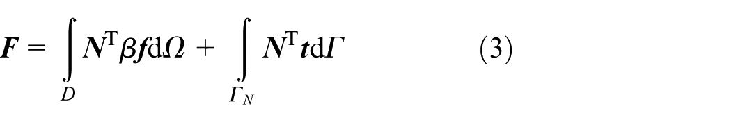
The FCM is a numerical analysis method within the fixed mesh and was proposed by Parvizian et al. ¹⁸ in 2007. The high-order Legendre shape function is adopted as the interpolation function in the FCM, and the quadtree/octree adaptive integral strategy is used to deal with mesh cutting by the structural boundary, which has a higher analysis precision. The analysis principle of the FCM is shown in Figure 1. For solving the problem of linear elastic mechanics in the structure domain Ω, the computing procedure is to first embed the considered structure of the physical domain Ω into a rectangular domain D and then to discretize D into a fixed mesh of finite cells. These cells can be classified into physical cells, virtual cells, and boundary cells. Then, using the variational principle, we obtain a system of differential equations

$$\mathit{KU}=\mathit{F}$$

(1)

where U is the displacement vector, and K and F are the stiffness matrix and the global load vector, respectively; therefore, the calculation formulas are given as

$$\mathit{K}=\underset{D}{\int }{\mathit{B}}^{\mathrm{T}}\beta \mathit{DB}\mathrm{d}\Omega$$

(2)

$$\mathit{F}=\underset{D}{\int }{\mathit{N}}^{\mathrm{T}}\beta \mathit{f}\mathrm{d}\Omega +\underset{{\Gamma }_N}{\int }{\mathit{N}}^{\mathrm{T}}\mathit{t}\mathrm{d}\Gamma$$

(3)

where B is the strain matrix, D is the elasticity matrix, D is only related to Young’s modulus and Poisson’s ratio, N is the matrix of the B-spline basis functions, and f and t are volume force vectors and boundary force vectors, respectively. The scalar factor β is defined as

$$\beta =\{\begin{array}{c}1.0\mathrm{in}\Omega \hfill \\ \multicolumn{1}{c}{0.0\mathrm{in}D\backslash \Omega }\end{array}$$

(4)

Figure 1.

Basic principle of the FCM and the quadtree refinement strategy.

In equations (2) and (3), the expressions of K and F are assembled by the stiffness matrix and load vector of the cell in actual calculation. The β value of all points inside the physical cell is 1, and the calculation method for the stiffness matrix and load vector is the same as that used in the traditional FEM. The β value of all points inside the virtual cell is 0, and the stiffness matrix and the load vector are zero matrix and zero vector, respectively. The β value of the points inside the boundary cell may be 1 or 0, so that we need to use the quadtree/octree refinement strategy to obtain highly encrypted gauss integral points along the structural boundary, and then the high-precision integral calculation of the material part could be carried out.

After obtaining the value of U from equation (1), the stress response under any point in the structure domain of ${\mathit{x}}_{\Omega }\in \Omega$ can be estimated

$$\mathbf{\sigma }\left({\mathit{x}}_{\Omega }\right)={({\sigma }_x\left({\mathit{x}}_{\Omega }\right),{\sigma }_y\left({\mathit{x}}_{\Omega }\right),{\tau }_{\mathrm{xy}}\left({\mathit{x}}_{\Omega }\right))}^{\mathrm{T}}=\mathit{DB}\left({\mathit{x}}_{\Omega }\right)\mathit{U}$$

(5)

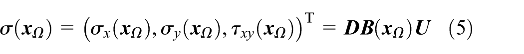
According to the three stress components, the von Mises stress of the ${\mathit{x}}_{\Omega }$ material point is defined as

$${\sigma }_{\mathrm{von}}\left({\mathit{x}}_{\Omega }\right)=\sqrt{\frac{{\tilde{\mathbf{\sigma }}}^{\mathrm{T}}\left({\mathit{x}}_{\Omega }\right)\tilde{\mathbf{\sigma }}\left({\mathit{x}}_{\Omega }\right)}{2}}$$

(6)

Here

$$\tilde{\mathit{\sigma }}\left({\mathbf{x}}_{\mathrm{\Omega }}\right)={\left({\sigma }_{\mathbf{x}}\left({\mathbf{x}}_{\mathrm{\Omega }}\right),{\sigma }_y\left({\mathbf{x}}_{\mathrm{\Omega }}\right),{\sigma }_{\mathbf{x}}\left({\mathbf{x}}_{\mathrm{\Omega }}\right)-{\sigma }_y\left({\mathbf{x}}_{\mathrm{\Omega }}\right),\sqrt{6}{\tau }_{\mathbf{x}y}\left({\mathbf{x}}_{\mathrm{\Omega }}\right)\right)}^{\mathrm{T}}$$

The core parts of the FCM are cell-type identification and quadtree/octree refinement. The effective implementation of the above steps involves quickly determining whether any point in the computational domain D is located in the structure domain Ω. For this purpose, we will use the implicit function to describe the structure domain Ω, and the relation between a point and Ω could be directly determined based on the sign (i.e. positive, zero, and negative) of the implicit function introduced in the next section.

Structural implicit model

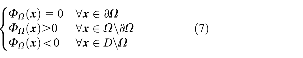
The structural implicit model, namely the implicit function, describes the structure domain Ω and can be written as Φ_Ω. Figure 2 shows an implicit model of the holed structure. As shown here, the Φ_Ω value related to a point outside the structure domain (i.e. the inner domain of the hole and the outer domain of the plate) is negative, and the specific expressions are written as follows

$$\{\begin{array}{c}{\Phi }_{\Omega }\left(\mathit{x}\right)=0\forall \mathit{x}\in \partial \Omega \hfill \\ \multicolumn{1}{c}{{\Phi }_{\Omega }\left(\mathit{x}\right)>0\forall \mathit{x}\in \Omega \backslash \partial \Omega }\\ \multicolumn{1}{c}{{\Phi }_{\Omega }\left(\mathit{x}\right)<0\forall \mathit{x}\in D\backslash \Omega }\end{array}$$

(7)

Combining the heaviside function H(•) with Φ_Ω, we can rewrite the β defined in equation (4) as

$$\beta =H\left({\Phi }_{\Omega }\left(\mathit{x}\right)\right)=\{\begin{array}{c}1\hfill \\ \multicolumn{1}{c}{0}\end{array}\begin{array}{c}{\Phi }_{\Omega }\left(\mathit{x}\right)⩾0\hfill \\ \multicolumn{1}{c}{{\Phi }_{\Omega }\left(\mathit{x}\right)<0}\end{array}$$

(8)

Figure 2.

Implicit model of the holed structure: (a) structural domain Ω and (b) implicit function Φ_Ω.

The construction method for the implicit function Φ_Ω is discussed below. On one hand, Φ_Ω is used for finite cell analysis within the fixed mesh to describe the complex geometry of the structure domain; on the other hand, it is used for shape optimization design to describe the free-variable hole boundary. For the former, this article uses the R functions, a type of implicit modeler with the rigorous theoretical foundation, to build Φ_Ω by Boolean operations. For the latter, this article uses the smoothly deformable implicit curve to describe the hole boundary. The most commonly used R function is defined as follows

$$\{\begin{array}{l}\multicolumn{1}{c}{{\Phi }_1{\wedge }_{\alpha }{\Phi }_2\equiv \frac{1}{1+\alpha }\left({\Phi }_1+{\Phi }_2-\sqrt{{\Phi }_1^2+{\Phi }_2^2-2\alpha {\Phi }_1{\Phi }_2}\right)}\\ \multicolumn{1}{c}{{\Phi }_1{\vee }_{\alpha }{\Phi }_2\equiv \frac{1}{1+\alpha }\left({\Phi }_1+{\Phi }_2+\sqrt{{\Phi }_1^2+{\Phi }_2^2-2\alpha {\Phi }_1{\Phi }_2}\right)}\end{array}$$

(9)

where Φ₁ andΦ₂ denote two implicit functions of the simple geometry; ∧ _α and ∨ _α , respectively, denote R-conjunction operator and R-disjunction operator, which correspond to the Boolean intersection operation ∩ and Boolean union operation ∪; α is the arbitrary function and satisfies the condition −1 < α ⩽ 1.

The construction method of the smoothly deformable implicit curve is inspired from the extended super-quadratic curve/surface proposed by Zhou and Kambhamettu. ¹⁹ The expression of the so-called super-quadratic curve is

$${\left|\frac{x}{a}\right|}^{2/\epsilon }+{\left|\frac{y}{b}\right|}^{2/\epsilon }=1$$

(10)

where a and b denote semi-axial lengths of the two main axes, and ε denotes the shape index. The extended super-quadratic curve has the ability to describe asymmetric structures by extending ε into polar angle functions in polar coordinate

$${\left|\frac{x}{a}\right|}^{2/f\left(\theta \right)}+{\left|\frac{y}{b}\right|}^{2/f\left(\theta \right)}=1$$

(11)

where θ is the polar angle in polar coordinate, and f(θ) is the continuous positive function of θ; f(θ) is constructed using Bernstein polynomials in the literature. ²⁰ However, it is inevitable that the extended super-quadratic curve in the deformation process goes through four points ((±a, 0) and (0, ±b)), which limits its expression ability and deformation ability to a large extent. In order to solve this problem, the smoothly deformable implicit curve is presented in this article by extending a and b into the function f(θ)

$${\left|\frac{x}{f\left(\theta \right)}\right|}^{2/\epsilon }+{\left|\frac{y}{f\left(\theta \right)}\right|}^{2/\epsilon }=1$$

(12)

Accordingly, the implicit function of the domain bounded by the smooth deformation implicit curve is as follows

$${\Phi }_S=1-({\left|\frac{x}{f\left(\theta \right)}\right|}^{2/\epsilon }+{\left|\frac{y}{f\left(\theta \right)}\right|}^{2/\epsilon })$$

(13)

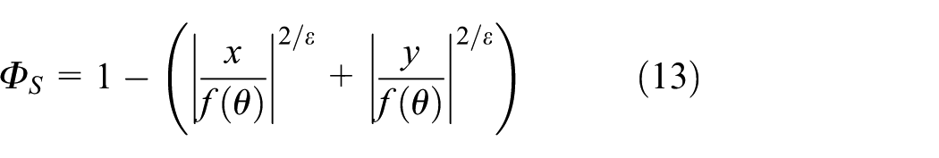
The polar angle θ can be expressed as a function of Cartesian coordinates (x, y)

$$\theta =\arctan \frac{y}{x}+\mathrm{sgn}(x)(\mathrm{sgn}(x)-1)\frac{\mathrm{\pi }}{2}$$

(14)

In equation (14), θ has a range of [–π/2, 3π/2). f(θ) in equation (13) can be determined using the B-spline basis functions

$$f(\theta )=\sum _{i=1}^n{N}_{i,p}\left(\xi \right)P_i=\sum _{i=1}^n{N}_{i,p}\left(\frac{\theta +\mathrm{\pi }/2}{2\mathrm{\pi }}\right)P_i$$

(15)

where N_{i, p}(ξ) is the B-spline basis function; n and p are the number and order of the B-spline basis functions, respectively; ξ is the parameter domain coordinate and its range is [0, 1); and P_i is a positive control parameter and satisfies the requirement P₁ = P_n = (P₂ + P_n−1)/2.

If the shape index ε in equation (13) is set to constant 1, then the smooth deformation implicit curve is simplified to the closed B-splines, as defined in the literature. ²⁰ At this point, in the polar coordinates shown in Figure 3(a), f(θ) is the polar radius corresponding to the polar angle θ. As shown in Figure 3, the adjustment of the control parameter P_i will lead to the change of f(θ), which achieves the purpose of changing the shape of the implicit curve.

Figure 3.

Smoothly deformable implicit curve (ε = 1): (a) polar coordinate system and (b) semi-major axis function f(θ).

Optimization model and sensitivity derivation

This study focuses on the shape optimization design of holed structures under different load boundary conditions. The optimization problem we address is minimizing the maximum von Mises stress when the volume of the structure is not increased. The mathematical model of the problem is as follows

$$\begin{array}{c}\multicolumn{1}{c}{\mathrm{Find}\epsilon ,P_2,P_3,\dots ,P_{n-1}}\\ \multicolumn{1}{c}{\mathrm{Min}\underset{{\mathit{x}}_{\mathit{\Omega }}\in \mathit{\Omega }}{\max }\left({\sigma }_{\mathrm{von}}\left({\mathit{x}}_{\mathit{\Omega }}\right)\right)}\\ \multicolumn{1}{c}{\mathrm{S}.\mathrm{t}.\mathit{KU}=\mathit{F}}\\ \multicolumn{1}{c}{V=\underset{D}{\int }H\left({\Phi }_{\Omega }\right)\mathrm{d}\mathit{\Omega }⩽V_{lim}}\\ \multicolumn{1}{c}{\epsilon >0,P_i>0i=2,3,\dots ,n-1}\end{array}$$

(16)

where V_lim is the given volume limit, and remaining parameters are defined as before. The shape index ε and control parameter P_i (i = 2, 3, …, n–1) are design variables, and they could be united into a vector $\mathit{v}=\{v_k{\}}_{k=1}^{n-1}=\{\epsilon ,P_2,P_3,\dots ,P_{n-1}\}$ .

The sensitivity of the von Mises stress ${\sigma }_{\mathrm{von}}({\mathit{x}}_{\mathit{\Omega }})$ to the variable v_k is

$$\frac{\partial {\sigma }_{\mathrm{von}}\left({\mathit{x}}_{\mathit{\Omega }}\right)}{\partial v_k}=\frac{1}{2{\sigma }_{\mathrm{von}}\left({\mathit{x}}_{\mathit{\Omega }}\right)}{\tilde{\mathbf{\sigma }}}^{\mathrm{T}}\left({\mathit{x}}_{\mathit{\Omega }}\right)\frac{\partial \tilde{\mathbf{\sigma }}\left({\mathit{x}}_{\mathit{\Omega }}\right)}{\partial v_k}$$

(17)

where the parameters are defined as before, and $\partial \tilde{\mathbf{\sigma }}({\mathit{x}}_{\mathit{\Omega }})/\partial v_k$ can be calculated as

$$\frac{\partial \mathbf{\sigma }\left({\mathit{x}}_{\mathit{\Omega }}\right)}{\partial v_k}=\mathit{DB}\left({\mathit{x}}_{\mathit{\Omega }}\right)\frac{\partial \mathit{U}}{\partial v_k}$$

(18)

where the elastic matrix D is only related to Young’s modulus and Poisson’s ratio, the strain matrix B is associated with the interpolation functions that are constant within the fixed mesh. Therefore, these two quantities are independent of the design variables. Moreover, this study does not involve the design-related load problem that the load F does not apply to the variable hole boundary, and thus, according to equation (1) we could obtain

$$\frac{\partial \mathit{U}}{\partial v_k}=-{\mathit{K}}^{-1}\frac{\partial \mathit{K}}{\partial v_k}\mathit{U}$$

(19)

with

$$\begin{array}{c}\multicolumn{1}{c}{\frac{\partial \mathit{K}}{\partial v_k}=\underset{D}{\int }{\mathbf{B}}^{\mathrm{T}}\mathit{DB}\frac{\partial H\left({\Phi }_{\Omega }\right)}{\partial v_k}\mathrm{d}\Omega =\underset{D}{\int }{\mathbf{B}}^{\mathrm{T}}\mathit{DB}\frac{\mathrm{d}H\left({\Phi }_{\Omega }\right)}{\mathrm{d}{\Phi }_{\Omega }}\frac{\partial {\Phi }_{\Omega }}{\partial v_k}\mathrm{d}\mathit{\Omega }}\\ \multicolumn{1}{c}{=\underset{D}{\int }{\mathbf{B}}^{\mathrm{T}}\mathit{DB}\frac{\partial {\Phi }_{\Omega }}{\partial v_k}\frac{1}{\Vert \nabla {\Phi }_{\Omega }\Vert }(\frac{\mathrm{d}H\left({\Phi }_{\Omega }\right)}{\mathrm{d}{\Phi }_{\Omega }}\Vert \nabla {\Phi }_{\Omega }\Vert )\mathrm{d}\mathit{\Omega }}\\ \multicolumn{1}{c}{=\underset{D}{\int }{\mathbf{B}}^{\mathrm{T}}\mathit{DB}\frac{\partial {\Phi }_{\Omega }}{\partial v_k}\frac{1}{\Vert \nabla {\Phi }_{\Omega }\Vert }\hat{\delta }\mathrm{d}\mathit{\Omega }=\underset{\mathit{\Gamma }}{\int }{\mathbf{B}}^{\mathrm{T}}\mathit{DB}\frac{\partial {\Phi }_{\Omega }}{\partial v_k}\frac{1}{\Vert \nabla {\Phi }_{\Omega }\Vert }\mathrm{d}\mathit{\Gamma }}\end{array}$$

(20)

In the equation, by introducing the Dirac delta function $\hat{\delta }$ (the directional derivative of heaviside function in the normal direction), the volume integral could be converted to the boundary integral. Similarly, the sensitivity of the structure volume V to the variable v_k could be obtained as

$$\frac{\partial V}{\partial v_k}=\underset{D}{\int }\frac{\partial H\left({\Phi }_{\Omega }\right)}{\partial v_k}\mathrm{d}\mathit{\Omega }=\underset{\mathit{\Gamma }}{\int }\frac{\partial {\Phi }_{\Omega }}{\partial v_k}\frac{1}{\Vert \nabla {\Phi }_{\Omega }\Vert }\mathrm{d}\mathit{\Gamma }$$

(21)

According to equations (20) and (21), the key to solving the sensitivity of the optimization model equation (16) is to calculate $\nabla {\Phi }_{\Omega }$ and $\partial {\Phi }_{\Omega }/\partial v_k$ . Φ_Ω is composed of the two types of implicit functions, one is integrated by basic geometries via the R functions, and the other is constructed by the smooth deformation implicit curves Φ_S. As the former is independent of the variable v_k, only the gradient and sensitivity of Φ_S need to be derived as follows

$$\nabla {\Phi }_S=\left(\begin{array}{c}\frac{\partial {\Phi }_S}{\partial x}\hfill \\ \multicolumn{1}{c}{\frac{\partial {\Phi }_S}{\partial y}}\end{array}\right)=\left(\begin{array}{c}\frac{2}{f(\theta )\epsilon }\frac{\partial f(\theta )}{\partial x}({\left|\frac{x}{f(\theta )}\right|}^{\frac{2}{\epsilon }}+{\left|\frac{y}{f(\theta )}\right|}^{\frac{2}{\epsilon }})-\frac{2}{\epsilon x}{\left|\frac{x}{f(\theta )}\right|}^{\frac{2}{\epsilon }}\hfill \\ \multicolumn{1}{c}{\frac{2}{f(\theta )\epsilon }\frac{\partial f(\theta )}{\partial y}({\left|\frac{x}{f(\theta )}\right|}^{\frac{2}{\epsilon }}+{\left|\frac{y}{f(\theta )}\right|}^{\frac{2}{\epsilon }})-\frac{2}{\epsilon y}{\left|\frac{y}{f(\theta )}\right|}^{\frac{2}{\epsilon }}}\end{array}\right)$$

(22)

$$\{\begin{array}{c}\frac{\partial f(\theta )}{\partial x}=-\frac{y}{x^2+y^2}\sum _{i=1}^n\frac{\mathrm{d}{N}_{i,p}}{\mathrm{d}\theta }{P}_i\hfill \\ \multicolumn{1}{c}{\frac{\partial f(\theta )}{\partial y}=\frac{x}{x^2+y^2}\sum _{i=1}^n\frac{\mathrm{d}{N}_{i,p}}{\mathrm{d}\theta }{P}_i}\end{array}$$

(23)

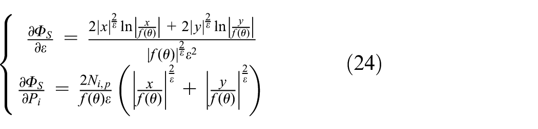
Considering the variable v_k could be the shape index ε or control parameters P_i, the sensitivity of Φ_S includes the following two forms

$$\{\begin{array}{c}\frac{\partial {\Phi }_S}{\partial \epsilon }=\frac{2{\left|x\right|}^{\frac{2}{\epsilon }}\ln \left|\frac{x}{f(\theta )}\right|+2{\left|y\right|}^{\frac{2}{\epsilon }}\ln \left|\frac{y}{f(\theta )}\right|}{{|f(\theta )|}^{\frac{2}{\epsilon }}{\epsilon }^2}\hfill \\ \multicolumn{1}{c}{\frac{\partial {\Phi }_S}{\partial P_i}=\frac{2N_{i,p}}{f(\theta )\epsilon }({\left|\frac{x}{f(\theta )}\right|}^{\frac{2}{\epsilon }}+{\left|\frac{y}{f(\theta )}\right|}^{\frac{2}{\epsilon }})}\end{array}$$

(24)

The numerical example

This section is based on the above theory and the optimization model. The shape optimization design of holed structures is carried out within the fixed mesh, the mechanics response is analyzed by the FCM, the hole boundary is represented using the smoothly deformable implicit curve, and the optimization algorithm named the method of moving asymptotes (MMA) ²¹ is adopted.

The four test boundary conditions are shown in Figure 4, and the materials as well as the geometric dimensions are the same. Moreover, the young modulus is 207.4 GPa, Poisson’s ratio is 0.3, and the plate thickness is 3 mm. The mesh of the holed structure are 40 × 40 cells; the upper volume limit V_lim was 4564 mm³, and 21 design variables (1 shape index and 20 control parameters) are set on the hole boundary.

Figure 4.

Four load boundary conditions: (a) uniform transverse tensile stress and longitudinal tensile stress, (b) uniform shear stress, (c) uniform transverse compressive stress and longitudinal tensile stress, and (d) triangularly distributed tensile stress.

Figure 5 shows the results of stress analysis of holed structures under four working conditions. Figure 6 shows the stress contour of the corresponding optimization results. As is clear from these figures, without increasing the volumes of the optimization results under the four working conditions, we reduced their maximum von Mises stresses by 35%, 18%, 24%, and 44%, respectively. Therefore, the stress concentration along the hole boundary decreases significantly.

Figure 5.

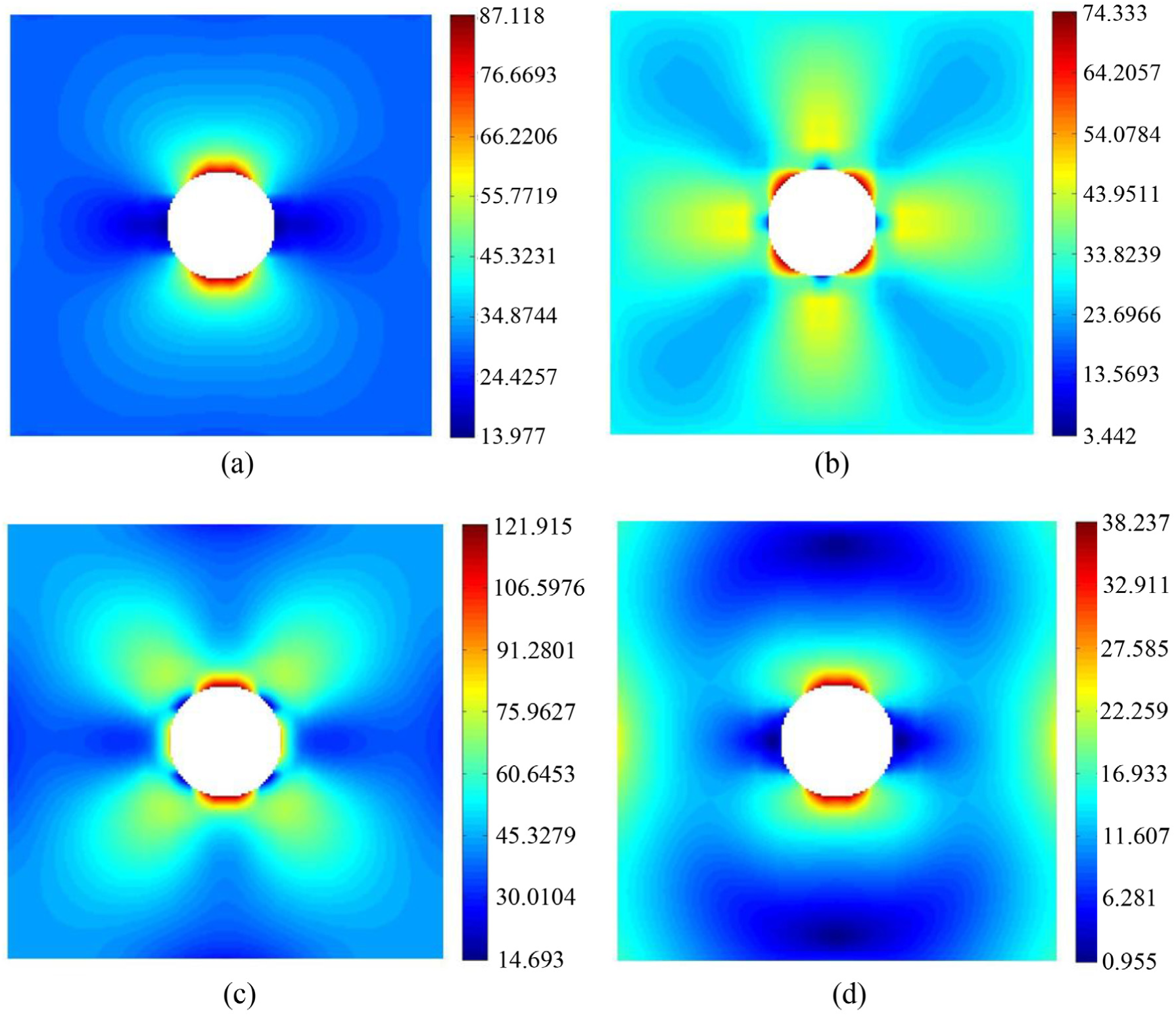
Stress analysis results under four load boundary conditions: (a) uniform transverse tensile stress and longitudinal tensile stress, (b) uniform shear stress, (c) uniform transverse compressive stress and longitudinal tensile stress, and (d) triangularly distributed tensile stress.

Figure 6.

Stress contours and hole shapes of optimized results under four load boundary conditions: (a) uniform transverse tensile stress and longitudinal tensile stress, (b) uniform shear stress, (c) uniform transverse compressive stress and longitudinal tensile stress, and (d) triangularly distributed tensile stress.

It is worth mentioning that the smoothly deformable implicit curve defined in this article has both advantages of the implicit form and the explicit form. In finite cell analysis, the implicit expression form of equation (13) is adopted to describe the hole boundary, so as to determine the location relation of the point and structural domain within the fixed mesh. During post-processes, the hole boundary was expressed in the following form to quickly solve the coordinates of the boundary point (x_S, y_S)

$$\{\begin{array}{c}{x}_S=f(\theta )\mathrm{sgn}\left(\cos \theta \right){\left|\cos \theta \right|}^{\epsilon }\hfill \\ \multicolumn{1}{c}{y_S=f(\theta )\mathrm{sgn}\left(\sin \theta \right){\left|\sin \theta \right|}^{\epsilon }}\end{array}$$

(25)

Equation (25) is equivalent to equation (13). The optimized boundaries of the holes shown in Figure 6 could be drawn conveniently according to equation (25). The results of the hole-shape optimization in Figure 6(a)–(c) are very close to the optimization results of the infinite perforated plate obtained by the analytical method in the literature. ²²

Conclusion

In this article, we focused on the hole-shape optimization of opening structures and presented a new optimization framework by combining the FCM and the novel implicit model, which could avoid the mesh update process existing in the traditional shape optimization method. It is helpful to expand the optimal design space to seek better solutions when the flexible and smoothly deformable implicit curve is adopted to describe the hole boundary. Numerical results show that this method can effectively reduce the stress concentration of the hole. If the outer boundary of the structure is also expressed using the smoothly deformable implicit curve, the approach presented in this article can optimize the shape of the whole structure. In future work, we will combine the isogeometric shell analysis with the proposed method to realize the collaborative optimization of the hole shape and the shell surface related to the opening shell structure.