
Abstract
In this article, a combined use of Latin hypercube sampling and axis orthogonal importance sampling, as an efficient and applicable tool for reliability analysis with limited number of samples, is explored for sensitivity estimation of the failure probability with respect to the distribution parameters of basic random variables, which is equivalently solved by reliability sensitivity analysis of a series of hyperplanes through each sampling point parallel to the tangent hyperplane of limit state surface around the design point. The analytical expressions of these hyperplanes are given, and the formulas for reliability sensitivity estimators and variances with the samples are derived according to the first-order reliability theory and difference method when non-normal random variables are involved and not involved, respectively. A procedure is established for the reliability sensitivity analysis with two versions: (1) axis orthogonal Latin hypercube importance sampling and (2) axis orthogonal quasi-random importance sampling with the Halton sequence. Four numerical examples are presented. The results are discussed and demonstrate that the proposed procedure is more efficient than the one based on the Latin hypercube sampling and the direct Monte Carlo technique with an acceptable accuracy in sensitivity estimation of the failure probability.
Keywords
Introduction
Reliability analysis and sensitivity analysis should be an important part of any analysis of engineering structures, with (1) reliability analysis providing the probabilities of failure or of unacceptable structural performance due to those uncontrolled random factors and (2) as an importance measure, sensitivity analysis identifying the contributions of random analysis inputs to those probabilities. In the framework of probability-based structural reliability analysis, an individual random input may be defined probabilistically by the probability density function (PDF) or cumulative distribution function (CDF) parameterized in terms of its probability characteristics such as mean (
Various reliability sensitivity analysis procedures have been proposed for use, including the most probability point (MPP)-based method,1,2 differential analysis,1,2 and sampling-based techniques.3,4 MPP-based method is simple, which gives the directions of the MPP in the standard normal space and provides sensitivities with respect to the MPP as its side product, but it depends on the linearization of limit state function, and the nonlinear performance function will result in a poor precision in the reliability and the reliability sensitivity estimation.2,5 Differential analysis is an indirect mathematical technique, whose precision is determined by the reliability analysis method itself. Sampling-based techniques are most adequate and employed for use in conjunction with Monte Carlo–type simulation methods including the standard Monte Carlo (SMC) simulation, importance sampling, quasi-random sampling 6 such as Latin hypercube sampling (LHS), random sampling with the Sobol sequence, Niederreiter sequence, and Halton sequence, and so on. The SMC simulation is often criticized for its time consumption and expensive computation cost especially calculating those small failure probabilities. Wu and Mohanty 7 suggested using a small number of random samples to compute sensitivities by classifying significant and insignificant random variables via acceptance limits derived from the test of hypothesis, without an approximation needed in either the form of the performance functions or the type of continuous distribution functions representing input variables. Lu et al. 8 proposed analyzing reliability sensitivity of a structural system based on the point estimation method for evaluating the first few moments of the system performance function. In the reliability-based optimization design, the dynamic Kriging method is used for surrogate models to reduce the computation cost and a stochastic sensitivity analysis is introduced to compute the sensitivities of probabilistic constraints with respect to independent or correlated random variables in the study of Lee et al. 9 A virtual support vector machine, as a classification method, is employed to evaluate a large number of Monte Carlo simulation (MCS) probabilistic sensitivity analyses for the same purpose in the study of Song et al. 10 Lin et al. 11 used the derivatives of response function incorporating with kernel density estimation for stochastic design sensitivity analysis. A local sampling method with variable radius is proposed to construct the Kriging model accurately and efficiently in the region of significance. 12 Besides, other importance measures are also discussed in the literature. Wu et al. 13 introduced an importance measure based on the component maintenance priority used to select components for preventive maintenance. An importance measure for both coherent and non-coherent systems is suggested defined on the change in mean time to failure caused by the failure (success) of a component in the study of Borgonovo et al. 14
LHS is very popular for use with computationally demanding models but only slightly more efficient than the SMC for evaluating small probabilities. 15 To solve this, Olsson et al. 16 investigated a combined use of LHS and axis orthogonal importance sampling for reliability analysis, and the method performs better than simple importance sampling using SMC and proves to be an efficient importance sampling strategy. However, it seems that the combined use of LHS and axis orthogonal importance sampling for reliability sensitivity analysis has not yet been thoroughly evaluated. In this article, we further focus on the numerical algorithm employing axis orthogonal importance Latin hypercube sampling (AOILHS) method to analyze the reliability sensitivities. As we know, the reliability sensitivities of the sampling-based method are evaluated as an expectation of the partial derivative of PDF with respect to the probability characteristics over the failure region. To verify the efficiency and accuracy of the proposed algorithm, it is compared to the other sampling-based methods in this article including the SMC method, axis orthogonal importance correlation Latin hypercube sampling (AOICLHS) method, and axis orthogonal importance sampling with the Halton sequence (AOIHalton) and illustrated by a number of numerical examples.
This article is structured as follows. The reliability analysis of AOILHS/AOICLHS is depicted in section “Basic idea of AOILHS/AOICLHS.” The reliability sensitivity estimator and its variance analysis based on AOILHS/AOICLHS are given in section “Reliability sensitivity estimation and variance analysis based on AOILHS/AOICLHS.” Numerical examples are shown and the efficiency and accuracy of the proposed algorithm are demonstrated in section “Numerical examples.” Section “Conclusion” concludes with a summary of the presented procedure.
Basic idea of AOILHS/AOICLHS
Importance sampling
Importance sampling proves to be an efficient variance reduction technique employed successfully in quite a few engineering fields. In the case of reliability analysis, the failure probability is calculated as the sum of a ratio

where
LHS
LHS is popularly employed for its efficient stratification properties with relatively lower computation while preserving the desirable probabilistic features of simple random sampling with a relatively small sample size.
A sample of size N in LHS is generated in the following manner from the target marginal distributions

where
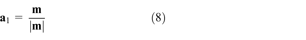
Unfortunately, there is a risk that some spurious correlation will appear in the primary generated sampling matrix

where

if the desired covariance equals to the identity, otherwise

where

Latin hypercubes in axis orthogonal importance sampling
Latin hypercubes can be applied in importance sampling in different ways. In this article, for comparison, only the simple Monte Carlo sampling method and the axis orthogonal importance sampling methods are considered.
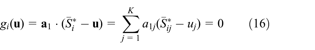
A LHS (CLHS) sample of the axis orthogonal importance sampling in the transformed normal space is established in the directions of the approximating tangent hyperplane (Figure 1). If the number of stochastic variables is K, the dimension of the tangent hyperplane is

where

(a) AIMC sampling and (b) AILHS/AICLHS sampling in the transformed normal space.
The remaining

More guidance on the

The Newton–Raphson algorithm in one dimension can be applied to find the solution, and a suitable start value for
Reliability sensitivity estimation and variance analysis based on AOILHS/AOICLHS
Reliability sensitivity estimation in the transformed standard normal space
The probability of failure with AIMC, AILHS, and AICLHS method is estimated by
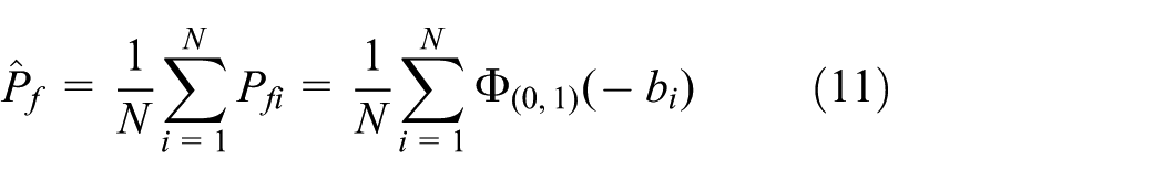
where

Since the samples generated in transformed normal space are independent and identically distributed (i.i.d.), the variance of the probability of failure can be calculated by

The reliability sensitivity of

where

In order to determine
where
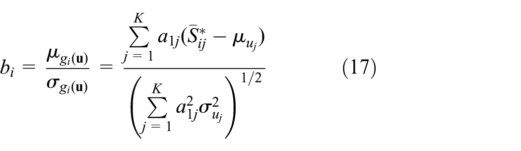
where

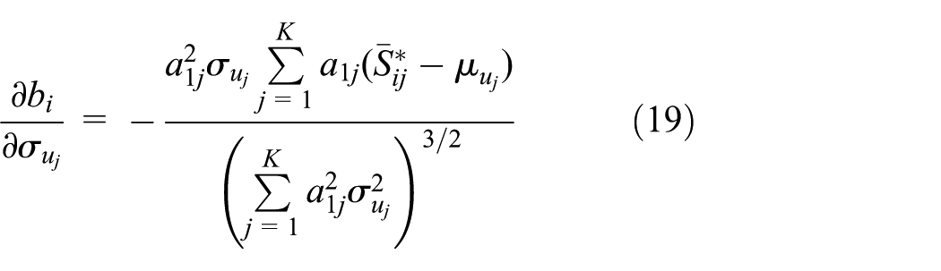
According to equations (14), (15), (18), (19), and considering

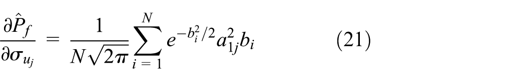
Equations (20) and (21) indicate that the reliability sensitivities can be simply determined by
Reliability sensitivity estimation when non-normal random variables are not involved
Usually, the parameter sensitivities with respect to
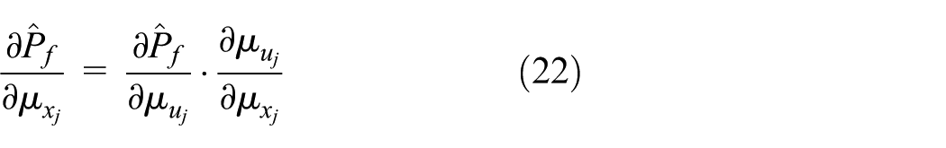

where

Thus,

Reliability sensitivity estimation when non-normal random variables are involved
There are no particular difficulties for the failure probability estimation using AOILHS/AOICLHS when non-normal random variables are involved, which is conducted in the same way as depicted in sections “Reliability sensitivity estimation in the transformed standard normal space” and “Reliability sensitivity estimation when non-normal random variables are not involved.” However, estimating the reliability sensitivities using AOILHS/AOICLHS is less straightforward. On the one hand, when non-normal random variables are involved, their transformations to the standard normal space applied in AOILHS/AOICLHS are usually non-linear, thus
Now the remaining effort is to estimate the reliability sensitivities directly upon the failure probability without taking derivatives, namely, the sensitivities of the failure probability to changes in the parameters. Considering the effect of changing one of the distribution parameters of a random variable, in the procedure of AOILHS/AOICLHS, small changes on the transformation of the random variable to normal space, the limit state function in normal space, and the failure probability associated with it will successively come into being. Thus, the reliability sensitivity can be calculated using finite difference method and written as

where
Reliability sensitivity variance analysis
First considering the variance of reliability sensitivities in the transformed normal space and since the samples generated in normal space are i.i.d, the variance of reliability sensitivities can be estimated by
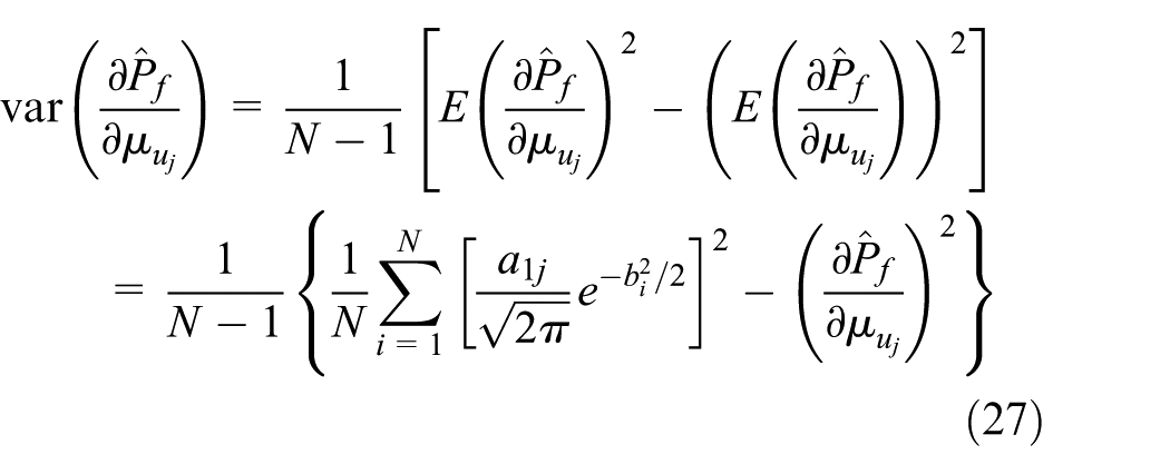

For those problems not involving non-normal random variables, variances of the reliability sensitivities can be calculated according to equations (22) and (23) and written as


For those problems involving non-normal random variables, variances of the reliability sensitivities can be calculated according to equations (11) and (26) and written as

Methodology
Now, the proposed procedure of AOILHS/AOICLHS for reliability sensitivity estimation can be summarized as follows:
Determine an approximate design point
Generate an
Transform each sample of
Each row of
For those problems in which non-normal random variables are not involved, calculate failure probability with equation (11) and reliability sensitivity according to equations (20)–(23). In the meantime, estimate the variances according to equations (27)–(30).
For those problems in which non-normal random variables are involved, calculate failure probability
Numerical examples
Four examples are illustrated below to demonstrate the computational efficiency and accuracy of the proposed reliability sensitivity estimation method based on the AOILHS, AOICLHS, and a representative quasi-random sampling strategy AOIHalton. For comparison, the failure probabilities (
Example 1
A non-linear limit state function with three independent normal random variables is considered.
2
The limit state function, basic random variables, and their distribution parameters are presented in Table 1. The mean value sensitivities (
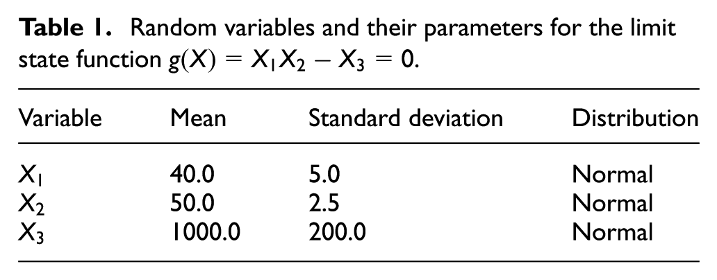
Random variables and their parameters for the limit state function
Sensitivities, failure probability, and reliability indices obtained from the AOILHS/AOICLHS.

AOILHS: axis orthogonal importance Latin hypercube sampling; AOICLHS: axis orthogonal importance correlation Latin hypercube sampling; SD: standard deviation; COV: coefficient of variation; SMC: standard Monte Carlo simulation.
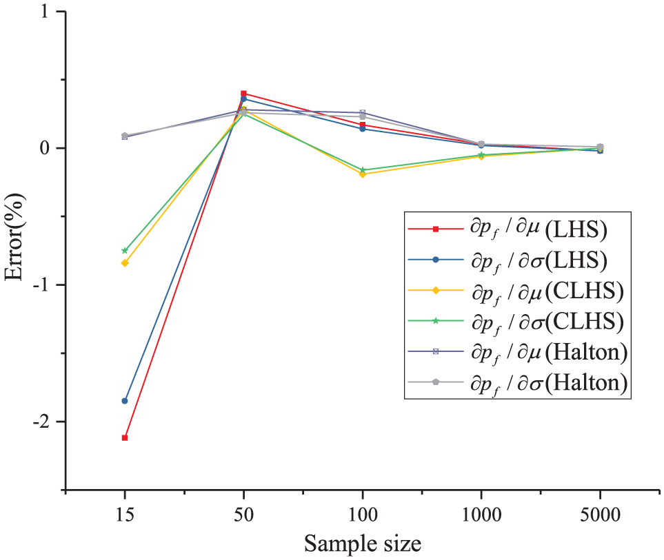
Relative errors of sensitivities with different sample sizes in example 1.
Example 2
A roof truss structural reliability problem is considered as shown in Figure 3.
27
The top chords and compression bars are made of steel-reinforced concrete, and the bottom chords and tension bars are made of steel. According to structural mechanics, the uniformly distributed load q applied on the roof truss can be equivalent to the nodal load

where
Distribution parameters of the basic random variables.

COV: coefficient of variation; SD: standard deviation.
Sensitivities, failure probability, and reliability indices obtained from the AOILHS/AOICLHS.

AOILHS: axis orthogonal importance Latin hypercube sampling; AOICLHS: axis orthogonal importance correlation Latin hypercube sampling; SD: standard deviation; COV: coefficient of variation; SMC: standard Monte Carlo simulation.

Schematic diagram of a roof truss: (a) under uniformly distributed load on roof truss and (b) under equivalent nodal loads.

Relative errors of sensitivities with different sample sizes in example 2.
Example 3
A highly non-linear limit state function involving both normal and non-normal basic random variables is considered. The limit state function, basic random variables, and their distribution parameters are presented in Table 5.
2
The mean value sensitivities (
Random variables and their parameters for the limit state function

Sensitivities, failure probability, and reliability indices obtained from the AOILHS/AOICLHS.

AOILHS: axis orthogonal importance Latin hypercube sampling; AOICLHS: axis orthogonal importance correlation Latin hypercube sampling; SD: standard deviation; COV: coefficient of variation; SMC: standard Monte Carlo simulation.

Relative errors of sensitivities with different sample sizes in example 3.
Example 4
A more complex 23-bar truss with 30 independent normal random variables is considered (Figure 6), including cross-sectional area for members, applied loads, and modulus of elasticity, whose distribution parameters are listed in Table 7. The limit state function is given based on vertical displacement of middle node


Truss structure with 30 random variables.
Random variables and their parameters in example 4.

Due to so many basic variables, only the relative errors of the mean value sensitivities and standard deviation sensitivities of the estimator with 50, 100, 500, 1000, and 10,000 samples compared to the exact ones determined with 1,000,000 samples based on AOICLHS are shown in Figure 7. The sensitivities with respect to the means and standard deviations of odd-numbered areas via different sampling methods are presented in Table 8. The failure probability and reliability index calculated by the FORM are
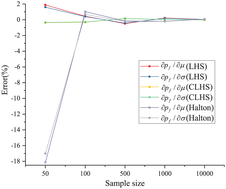
Relative errors of sensitivities with different sample sizes in example 4.
Sensitivities with respect to the means and standard deviations of odd-numbered areas via different sampling methods.

AOILHS: axis orthogonal importance Latin hypercube sampling; AOICLHS: axis orthogonal importance correlation Latin hypercube sampling; AOIHalton: axis orthogonal importance sampling with the Halton sequence; ILHS: importance Latin hypercube sampling; SMC: standard Monte Carlo simulation.
Discussion
The proposed procedure for reliability sensitivity estimation based on the axis orthogonal importance sampling methods (AOILHS, AOICLHS, and AOIHalton) is, as the previous examples indicate, considerably more efficient than the simple Monte Carlo sampling methods with relatively little computational cost. The variance-reduction effect of using the AOICLHS instead of the AOILHS, even the AOIHalton, results in better parameter sensitivity estimation especially under small sample size. The results obtained from the AOICLHS, AOIHalton, and AOILHS have a smaller difference as the sample size increases to some extent.
The proposed method can be employed to estimate reliability sensitivities with an acceptable degree of accuracy, which is demonstrated by a variety of the above nonlinear limit state functions including a normal and non-normal random variables involved case. The sensitivity estimation is closely similar to the results obtained from the direct simple Monte Carlo or simple Monte Carlo–based analysis. The involved non-normal random variables have a significant effect on reliability sensitivity estimation especially for some varieties of non-normal distributions and may produce more errors, for example, the mean value sensitivity estimation
Conclusion
This article demonstrates the axis orthogonal Latin hypercube importance sampling as an efficient and applicable tool for reliability sensitivity analysis. The Latin hypercube sample is established around near the MPP and in the directions of the approximating tangent hyperplane of limit state surface. The Newton–Raphson algorithm in one dimension is applied to find a coordinate value in the local coordinate system of the intersection point with limit state surface for each realization of a sampling plan, which is used in the following reliability analysis. Two versions of axis orthogonal Latin hypercube importance sampling with and without reduction in spurious correlation (AOICLHS and AOILHS) and an AOIHalton are applied and discussed in the parameter sensitivity estimation. The results obtained from the numerical examples show that the presented procedure is superior in computation cost with a relatively small sample size compared with the LHS and Monte Carlo method while preserving an acceptable accuracy.
Footnotes
Acknowledgements
Jiaming Cheng is gratefully acknowledged for his data processing of the complementary figures and tables in the revised manuscript.
Handling Editor: Xihui Liang
Declaration of conflicting interests
The author(s) declared no potential conflicts of interest with respect to the research, authorship, and/or publication of this article.
Funding
The author(s) disclosed receipt of the following financial support for the research, authorship, and/or publication of this article: This work was jointly supported by the NSFC (nos 11402097, 11272361, and 51278226) and the National Plan for Science and Technology Support of China (no. 2012BAJ07B02).