Sage Journals: Discover world-class research

Abstract

The problem of state-space explosion and state reachability decision has been a focus in Petri net analysis. In this article, some algorithms based on data features of state space are proposed for state-space reduction and reachability analysis in Petri nets. A caching arrangement algorithm for the state reachability graph is proposed to alleviate the memory overhead when all states are generated by a traditional reachability graph generation algorithm. For the reduction of the state space, a compression algorithm based on a hybrid coding is formulated. The changing characteristics of state elements are fully utilized to realize a sharp reduction of the whole state space. For the state reachability analysis, a state reachability retrieval algorithm based on the locally sensitive hashing is reported. In this algorithm, all the states in the compressed state space are distributed to different hash buckets according to the distances among the states, which realize the primary state retrieval efficiently. Then, a state retrieval strategy that reverts the primary retrieved state to its original data is adopted. Finally, the proposed compression and retrieval algorithms are validated on several Petri net models, showing high compression efficiency and exact accuracy of state retrieval.

Keywords

Petri net state-space compression predictive coding hashing retrieval state reachability

Introduction

Petri nets, a formal modeling tool invented by CA Petri,¹ have been applied to many fields, such as control of discrete event systems,^2–17 system reliability analysis,^18–23 modeling, analysis, control,^24–33 and the verification of communication protocol.³⁴ In the analysis of Petri nets, state-space techniques are used in marking reachability, forbidden states including deadlock control,^35–37 opacity verification and enforcement, and fault diagnosis.^27,38–45 Unfortunately, the size of a state space has a tendency of growing exponentially with respect to the structural scale of a Petri net, which is known as the state-space explosion problem (S²EP).⁴⁶ It hinders the development and applications of Petri nets due to the limited capacity of a real computer system in processing a large-size state space. Meanwhile, the state reachability analysis (SRA) is the most fundamental dynamic issue of a discrete event system; many other properties or problems of discrete event systems, such as the deadlock prevention, supervisory control design, and fault diagnosis, can be converted into the reachability problem. The state-space compression and reachability analysis methods show vital significance to alleviate the state-space explosion and analyze the pertinent properties of Petri nets.

Much work concerning state-space compression or reduction has been done to tackle the S²EP.⁴⁷ The study in Schmidt⁴⁸ uses place invariants and transition invariants to construct the state space of a Petri net. The place invariants which reduce the number of places of every marking show superiority over time and space. Meanwhile, the transition invariants which decrease the number of markings present a slight strength in space with low time efficiency. However, combined with the partial-order compression method, transition invariants in Schmidt⁴⁸ manifest a remarkable improvement in space and time.

A partial-order reduction⁴⁹ method exploits the independence of concurrently executed events to address the S²EP. It reduces the size of reachable state set by a cycle constraint and allows portions of the state space to be pruned. The method usually shows satisfactory performance in memory consumption. The minimal coverability sets method by Piipponen and Valmari⁵⁰ deals with two key problems to construct minimal coverability sets. One is to explore conditions or criteria under which a marking is converted to a finite coverability set of reachable markings. Another is to preserve the maximal coverability set with data structures based on binary decision diagrams and covering sharing trees. The method presents excellent time efficiency, but its internal memory consumptions are huge.

In Clarisó et al.,⁵¹ an abstract interpretation method is proposed. It includes two abstract domains and uses linear inequalities and polynomial equalities to derive non-structural invariants. The abstract interpretation has good performance in the state-space reduction but poor reachable state verification. The work in Emerson and Wahl⁵² proposes a dynamic symmetry reduction method by using a symbolic algorithm to generate the reachable state set. In the light of the symmetry of the fired path among states, the algorithm calculates dynamically respective representation symbols of states and ensures the uniqueness between symbols. While the state reachability graph is generated, states are sequentially mapped to their representative symbols. Finally, all the reachable states are equivalently characterized by representative symbols to achieve the reduction of state space.

The transitions merging method by Kurshan et al.⁵³ compresses a sequence of transitions into a single transition to eliminate the interim states. The authors of Bozga et al.⁵⁴ apply a live variable reduction method to construct equivalence representations on a system model by dead values unused either in variables or in queue contents, which simplifies the state space with a rather considerable ratio.

McMillan⁵⁵ proposes a net unfolding method that constructs a finite prefix by unfolding the net and forms an occurrence net. The unfolding will be ceased when the occurrence net structure generated is sufficient to characterize all the reachable markings. This occurrence net, simplifying the overlapping transitions among concurrent events, avoids the state explosion problem in the process of searching the whole state space. In view of the fact that the finite prefix constructed in McMillan’s net is too large, an improved method is proposed in Esparza et al.⁵⁶ The method makes the number of non-truncated events less than the total number of reachable states by employing the adequate orders, which can effectively realize the reduction of the state space.

In general, previous works present the high compression efficiency with varying degrees, which are usually based on a good understanding of the structure of Petri nets. Meanwhile, these compression methods may confront with a complicated search issue and data structures issues based on the reachability graph and net structure. The S²EP and SRA problems are coupled with each other and the methods of the state compression and state retrieval must be considered systematically. A universal compressed and retrieval method is credible, which does not involve the complex structure of Petri nets.

In this article, focusing on data characteristics of the state space in Petri nets, we propose three algorithms to deal with the S²EP and SRA problems. First, a caching arrangement algorithm for the efficient generation of state reachability graph is proposed. Then, to reduce the state space, a compression algorithm based on the hybrid coding is proposed, in which every state is compressed. Finally, for the SRA, we propose a state reachability retrieval algorithm based on the locally sensitive hashing algorithm, which implements data classification on the basis of the distance similarity and achieve highly efficient data retrieval.

The rest of this article is organized as follows. Section 2 introduces the basic concepts of Petri nets. The proposed caching arrangement of the reachability graph method is described in section “Caching arrangement of the reachability graph algorithm” in detail. Section “Basic methods on data compression and retrieval” presents some basic methods in data compression and retrieval for a better understanding of the reported algorithm. The proposed compression method is described in section “State-space compression based on hybrid coding.” In section “State reachability retrieval based on locally sensitive hashing,” a state retrieval algorithm is developed. The experimental results are given in section “Experiment” and the conclusions are reached in section “Conclusion.”

Petri nets

A Petri net is a four-tuple N = (P, T, F, W), where P = {p₁, p₂, …, p_m} is a non-empty finite set of places drawn by circles in which the number of black dots indicates the amount of tokens in a place, and T = {t₁, t₂, …, t_n} is a non-empty finite set of transitions drawn by rectangles with P∩T = ø, and F ⊆ (P × T)∪(T × P) represents a flow relation drawn by arcs with arrows from places to transitions or from transitions to places. W: (P × T)∪(T × P) → N is a mapping that allocates a weight to an arc: W(x, y) > 0 if (x, y) ∈ F, and W(x, y) = 0 otherwise, x, y ∈ P∪T and N = {0, 1, 2, …, } is a set of non-negative integers.

A marking M called a state of a Petri net N is a mapping P to N, where M(p) denotes the number of tokens in place p. (N, M₀) is called a net system or marked net with an initial marking M₀. A marking M is usually represented by a |P|-dimensional vector M = [M(p₁), M(p₂), …, M(p_|P|)] that indicates token distribution of all places.

A transition t ∈ T is enabled at M, which is denoted as M [t〉, if M(p_i) ≥ W(p_i, t) for any p_i ∈ •t. Then, a new marking M′, defined by M′ (p_i) = M(p_i) − W(p_i, t) + W(t, p_i), for p_i ∈ •t, is reached by firing t from M. The fact is denoted as M[t〉M′. Marking M′ is said to be reachable from M if there exist a sequence of transitions σ = t₀, t₁, …, t_n and markings M₁, M₂, …, M_n such that M [t₀〉M₁[t₁〉M₂,·…,·M_n [t_n〉M″ holds. The set of markings reachable from M in N is called the reachability set of Petri net (N, M) which is denoted as R(N, M). The state space of a Petri net N consists of all reachable markings from the initial marking M₀.

The state space of Petri nets N can be represented as an m × n matrix M,⁵⁷ where

The first row denotes the initial marking M₀.

Every row in matrix M represents a reachable marking from the initial marking M₀ except the first row.

All rows in matrix M are different from each other.

The matrix M containing all reachable markings fully characterizes the state space of a Petri net N. Given a marking M′, if it can be found in matrix M, then M′ is reachable from the initial marking M₀ in the Petri net. The analysis of the marking reachability in Petri nets is equivalent to a retrieval issue.

A Petri net example is presented in Figure 1(a). It consists of five places P = {p₁, p₂, p₃, p₄, p₅}, six transitions T = {t₁, t₂, t₃, t₄, t₅, t₆}, and the initial marking M₀ = (1, 0, 0, 0, 0). Its state-space reachability graph⁵⁷ is shown in Figure 1(b). The state space composed by all markings can be represented by a 5 × 5 matrix M presented in Figure 1(c). In M, every row denotes a marking.

Figure 1.

A simple Petri net model. (a) A Petri net example. (b) The state-space reachability graph of the Petri net ((a)). (c) The state space of the Petri net described in matrix M.

If any marking can be found from the rows in matrix M, the marking is reachable from the initial markings M₀ in the state space. For example, given a marking M′ = (0 0 1 0 0), it can be found in M, indicating that M′ is reachable from M₀.

Caching arrangement of the reachability graph algorithm

For the study of the state space in a Petri net, the traditional process⁵⁸ is to generate the whole state space, named the original data in this article, and then conduct the subsequent compression process. When the scale of a state space reaches a certain degree, the reachability graph is hardly possible to be stored due to the limited memory.⁵⁹ The relationship between the state count and the number of philosophers in the classic dining philosopher systems (DPS⁶⁰) is shown in Figure 2, where the drastic increase in the system brings state explosion, which leads to block the study of the state compression itself.

Figure 2.

State-scale counts of DPS with the number of philosophers.

In order to alleviate the storage issue caused by the state explosion before compressing the state space, a caching arrangement algorithm of the reachability graph shown in Table 1 is proposed as follows.

Table 1.

The caching arrangement algorithm of the reachability graph.

Input: Petri net (N, M₀)
Output: The caching blocks of reachable states RS₁(N, M₀), RS₂(N, M₀), …, RS_n(N, M₀)

1. Initializing the root vertex M₀ and it is not labeled at the initial time instance
2. Initializing the counter of reachable States n and the maximum caching states MaxNum
3. Initializing the current caching block of reachable states i = 14. Setting a caching region R
5. While {the unlabeled vertex is found} do
6. Denote the unlabeled vertex as M
7. For every transition t in M,
$M' = M + [N] (., t)$

✓ 8 if {the vertex M′ is not in the reachability graph}, then
✓ 9 Add the vertex M′ to the reachability graph
✓ 10 Record M′ in R
✓ 11 Add the arc from M to M′
✓ 12i = i + 1
✓ 13 if {MaxNum == i}, then
✓ 14 Reading out all state data as RS_i(N, M₀) in R and empting R.
✓ 15 end if
✓ 16 end if
✓ 17 Add the label “old” to M
✓ 18 end while

In Table 1, each unlabeled reachable state M is enabled and fired to generate a new marking M′, and the state M′ will be stored in the caching region. Once the number of states stored in the caching region reaches the MaxNum, all the states in the caching region will be extracted for the subsequent state compression process. Then, the caching region is cleared. The above procedure is conducted circularly until the whole reachability graph has been gained. The algorithm depends on equation $M' = M + [N] (., t)$ , which includes a counter and an addition operation. The algorithm complexity is O(n), where n is the counter of reachable states. The caching arrangement algorithm of the reachability graph is a useful solution to the state storage problem caused by the state explosion, which makes the study of the large-scale Petri nets possible.

Basic methods on data compression and retrieval

The methods of data compression consist of lossy and lossless based on the degrees of information distortion. A lossy compression method is mainly applied in a low accuracy scene and can reach a good compression efficiency. In comparison, the lossless compression has a low compression efficiency, but meets a high-accuracy requirement. In this article, we focus on the lossless compression. The proposed method of data compression consists of the Run-Length Encoding (RLE), Golomb–Rice coding, and adaptive prediction encoding, while the retrieval method is the locally sensitive hash (LSH), and the measure method in data retrieval utilizes hamming distance.

The RLE

The RLE^61,62 based on the statistical coding is considered as a lossless data compression technique. In the RLE, the same values that occur in many consecutive elements are stored as the ordered pairs $(g_{k}, l_{k})$ , a single value $g_{k}$ , and count $l_{k}$ . A concrete example of the RLE is shown in Figure 3.

Figure 3.

A run-length coding principle example.

In Figure 3, a string of 18-bit 300000000011110000 has four runs (3, 1), (0, 9), (1, 4), and (0, 4). It is encoded as 8-bit 31091404 by the RLE. The RLE traces element values and its counts of strings by sequential scanning.

The Golomb–Rice coding

The Golomb–Rice coding,^63,64 conducted mainly for non-negative integers, is a data compression method without loss of information in the coding process. The main idea of the Golomb–Rice coding is to use shorter encodings for smaller numbers and use longer encodings for larger numbers, that is, if the encoded value is smaller, the coding length is shorter. It achieves the purpose of data compression and saves the storage space.

The Golomb–Rice coding uses an adjustable parameter m and a block encoding method, by which the input string x is divided into two parts consisting of the group number q and the remaining part r. q and r can be calculated by the following formulas. The symbol % denotes the remainder operator

q = \frac{x}{m}

(1)

r = x % m

(2)

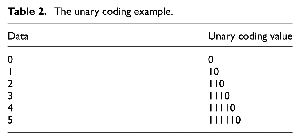
After the input string x is divided, a unary coding is used for encoding q. The unary coding is a simple encoding method for non-negative integers only. Given a non-negative integer num, its unary coding is composed of num “1” plus “0.” An encoding example is given in Table 2.

Table 2.

The unary coding example.

Data	Unary coding value
0	0
1	10
2	110
3	1110
4	11110
5	111110

Meanwhile, a fixed-length binary coding is conducted to encode r, which means that the low $\log_{2} (m)$ bits are served as the encoding value of r. The parameter m is usually set to an integral power of 2. In the end, the Golomb–Rice coding of x is constructed by the combination of the unary coding of q and the binary coding of r.

The adaptive prediction encoding

The main idea of the predictive coding^65,66 is described as follows. First, a mathematical model is established to predict the current sample point by using historical sample data, and then, the difference value is obtained by subtracting the current actual value by the predicted value. As a result, the difference value that is relatively small can be encoded to achieve the compression purpose. The predictive coding diagram is shown in Figure 4.

Figure 4.

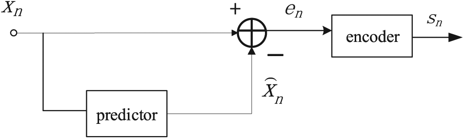
The component diagram of the predictive coding.

The predictor forecasts value x_n that is currently being encoded through the previously encoded data. Thus, the predicted value ${\hat{x}}_{n}$ is obtained. The difference value is called an error e_n of x_n, which is compressed by the encoder to obtain the ultimate value s_n.

The adaptive predictive coding⁶⁷ is a nonlinear prediction method. In the processes of data prediction, the adaptive prediction method corrects and adjusts constantly the predictive coefficient by analyzing the statistic characteristic and the variation of the original data, which makes the predictor change with the input data and obtains the ideal output of the predicted value finally. The schematic diagram is shown in Figure 5.

Figure 5.

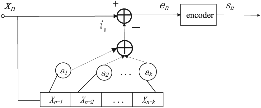
The component diagram of the adaptive predictive coding.

In Figure 5, the current sample x_n is predicted by the nonlinear combination of some sample X_n–₁, X_n–2, …, X_n-k before the current coding. The predictive value formula of the adaptive predictive coding is shown as follows

{\hat{x}}_{n} = \sum_{i = 1}^{k} a (i, n) X_{n - i}

(3)

where the predictive coefficient a(i, n) is related to the information source X_n-i. After the predictive value is achieved, the error value e_n can be subsequently computed by equation (4)

e_{n} = x_{n} - {\hat{x}}_{n} = x_{n} - \sum_{i = 1}^{k} a (i, n) X_{n - i}

(4)

The error value e_n is the difference value between x_n and its predicted value ${\hat{x}}_{n}$ , and e_n is eventually encoded as s_n by the encoder when the adaptive predictive coding finishes. The adaptive predictive coding makes full use of the characteristics of data change, and its output can better reflect the current sample characteristics.

LSH

As an efficient approximate query method, the locally sensitive hash (LSH)^68,69 is applied to mass data query. For a given mass data set, the set is chronologically mapped into binary codes called the hash value by a series of hash functions h_i() (i = 1, 2, …, n). The nearer data are hashed to the same hash value named the hash bucket by a large probability. As a result, the query efficiency can be much improved. The LSH schematic diagram is shown in Figure 6.

Figure 6.

The LSH schematic diagram.

For a series of hash functions H = {h₁(), h₂(), …, h_n()}, H is a mapping from the original data set X to the hash code space U, that is, $H = {h : X \to U}$ . For any two points p, q, D(p, q) is the distance measurement function of p and q. If the following conditions are satisfied, H is said to be (r₁, r₂, p₁, p₂) sensitive

If $D (p, q) \leq r_{1}$ , $P [h (q) = h (p)] \geq p_{1}$

If $D (p, q) > r_{2}$ , $P [h (q) = h (p)] \leq p_{2}$

$p_{1} > p_{2}$ , $r_{1} < r_{2}$

In the above, P [.] denotes the probability of mapping the two points to the same hash bucket. The LSH definition indicates the probability relation of the data distance. The relationship curve of the distance and the probability is shown in Figure 7.

Figure 7.

Probability with the data distance.

As shown in Figure 7, the distance versus probability curve is a monotonous decline. The key segment is the critical distance between r₁ and r₂. When the distance is greater than r₁, the probability of mapping into the same hash bucket is very high and greater than p₁, but it is rather minute-less than p₂, when the distance is less than r₂. Therefore, the main focus is just on the interval between (0, r₁) and (r₂,+∞).

Hamming distance

Hamming distance,⁷⁰ mainly implemented by adding up the sum of different values in the same location between two code words, is a measure methodology of the distance similarity. If X and Y are two code words with their length being n, the hamming distance is defined as follows

D_{HD} (X, Y) = \sum_{i = 1}^{n} x_{i} \oplus y_{i}

(5)

In equation (5), x_i denotes the ith bit value of the code word X and ⊕ represents the XOR, $x_{i} \in {0, 1}$ , and $y_{i} \in {0, 1}$ . The hamming distance is an efficient similarity measurement and suitable for the distance measurement of binary codes.

State-space compression based on hybrid coding

From the view of data characteristic, if the state space of a Petri net is represented as a matrix M composed of reachable state vectors, the reduction of the state space is equivalent to the compression of the state-space matrix M.

For every element in M, the current element value and its local adjacent element value usually manifest a stable and continuous variation, that is, during the firing of the transition tokens in places of discrete flow, and the number of tokens of only a few places will change. The state-space matrix M of a flexible manufacturing system is shown in Figure 8. State 2 is reachable from state 1 when some transitions fire, in which the tokens of most places between state 1 and state 2 remain unchanged.

Figure 8.

State-space matrix M of a flexible manufacturing system.

Motivated by the variation property of M, a state-space compression algorithm based on hybrid coding is proposed in this article, which consists of two compression modes, namely, the run-length coding and predictive coding. First, the current state is compressed in accordance with the local difference values between the current element and its adjacent element in M. Then, the traditional run-length coding method is used when local difference values of the current element are zero. In addition, a predictive coding method is adopted. At the same time, the error value in the prediction coding is compressed by the Golomb coding method. The flow diagram of the proposed algorithm is shown in Figure 9.

Figure 9.

Flow diagram of the state-space compression algorithm based on hybrid coding.

Computation of local difference values

Since the elements in M are encoded sequentially, the context of the current element needs to be determined for choosing a proper encoding mode and laying the foundation of the predictive encoding mode. The context of current encoding element x, that is, the neighborhood of x, has a–d five elements and is illustrated in Figure 10.

Figure 10.

Illustration of the context.

In Figure 10, the adjacent elements a, b, c, d, and e of the current encoding element x constitute the context of x, which implies the characteristics of local data variability of x. The difference values g_i (i = 1, 2, 3, 4) between x and its adjacent elements are given as follows

g_{1} = d - b

(6)

g_{2} = b - c

(7)

g_{3} = c - a

(8)

g_{4} = b - e

(9)

The difference values g_i can effectively decide the variation intension of x’s adjacent elements and make a preparation for the subsequent encoding mode choice and the predictive value computation in the predictive encoding mode.

Encoding mode selection

Through the computation of the adjacent difference value g_i of the current element, the encoding process enters the coding mode selection phase. The encoding mode selection process is shown in Figure 11.

Figure 11.

Flow diagram of the encoding mode selection process.

If the difference value g_i is zero, the algorithm chooses the predictive coding mode where the location variation of the element x is active; otherwise, it chooses the RLE code where x′ local variation is steady and continuous.

The predictive value computation

The data model is generally built via the characteristic of the adjacent elements of the current sample by traditional adaptive predictive encoding method.⁷¹ However, the algorithm complexity is high using this method. In this article, a first-order edge detection mechanism is employed to compute the predictive value during the predictive encoding, which achieves a good predictive effect with low complexity. The predictive value $\hat{x}$ of the current encoding element x can be implemented by the following formula (10)

\hat{x} = {\begin{matrix} min (a, b), c \geq \max (a, b) \\ max (a, b), c \leq min (a, b) \\ a + b - c, else \end{matrix}

(10)

For the context in Figure 10, the predictive value computation is conducted by choosing the maximum among a, b and a + b − c. The most outer elements e and d of x are not used in the predictive value computation. This makes the computation simpler and more effective.

RLE mode

The RLE mode⁷² is executed when the data set vary consistently.

State reachability retrieval based on locally sensitive hashing

From the perspective of matrix M, the state reachability retrieval in Petri nets state space is equivalent to the data retrieval issue. The state reachability retrieval algorithm based on locally sensitive hashing is proposed in this article. This algorithm innovatively introduces locally sensitive hashing applied in data retrieval for the SRA. The realization procedures of the algorithm are shown in Figure 12.

Figure 12.

The procedure block diagram of the proposed state reachability retrieval algorithm.

Normalization of state length

Since the lengths of compressed states are unfixed by the previous hybrid coding algorithm, we need to make the lengths of states consistent before applying the locally sensitive hashing method. First, the maximal length Lmax is given by equation (11)

Lmax = \max (length (M_{i})) (i = 1, \dots, n)

(11)

where n denotes the count of reachable states and M_i represents the ith state. The functions length() and max(), respectively, denote the calculation of the vector dimension and the maximum value. When the length of a state in the state space is less than Lmax, we append zero element to the state such that the state lengths are constant in the end.

Establishing the hash index structure

Constructing an effective index structure is a key point in LSH algorithm, which can achieve an efficient query of given states. The aim of constructing the index structure is to acquire hash functions.

Given p = (x₁, x₂, …, x_n), the hamming code of p is defined as follows⁷³

v (p) = Unar y_{k} (x_{1}) Unar y_{k} (x_{2}) \dots Unar y_{k} (x_{n})

(12)

where Unary_k(x_i) denotes that the first x_i bits are 1 and v(p) is the combination of the sequence Unary_k(x₁), …, Unary_k(x_n).

Any one of hash functions h can be constructed by the following method

h (m) = {\begin{matrix} 0, \\ 1, \end{matrix} \begin{matrix} r (v (m)) = 0; \\ otherwise \end{matrix}

(13)

where r() means rth bit of v(m) and r is the random integers subjected to the uniform distribution. The hamming code of state m is denoted as v(m). This random construction of hash functions in locally sensitive hashing is handler and more applicable.

The compressed state space M = {M₀, M₁, …, M_n} is the queried data set. First, a series of random hash functions h_i(.) are generated to initialize l hash tables. After the initialization of hash tables is finished, states M_i are mapped into different hash buckets by hash functions. The constructing of the hash index structure mainly classifies the state set and reduces dimensions of states, which contributes to an efficient state query in the next.

Primary state retrieval

After the index structure of M is constructed, the near states are mapped into the same hash bucket. For a given state q, q is mapped into No. h′(q) hash bucket by a random hash function h′(q). Therefore, all the states in No. h′(q) hash bucket are similar to q. In the end, states in No. h′(q) hash bucket are sorted by the distance measure, and the candidate state S₁ is queried to achieve the primary state retrieval.

Fine retrieval by returning

An unreachable state can be retrieved from the state space by a mistake, since the unreachable state or the retrieved state may be mapped into the same hash bucket. Therefore, an accurate state retrieval is introduced via returning the retrieved state q and the candidate state S₁ to their original states Q_in and M_in, that is,. the states before being hashed. Then, M_in and Q_in are compared to decide whether they are equal. If M_in and Q_in are equal, the retrieved state q is a reachable state. The fine state retrieval method realizes accurate reachability analysis with little time consumption.

Experiment

Experiment models

This section conducts experiments to discover the state-space compression ratio and state retrieval time by applying the proposed methods. The first experiment is devoted to a Petri net model of a flexible manufacturing cell that consists of 26 places p₁–p₂₆ and 20 transitions t₁–t₂₀.⁷ The model shown in Figure 13 can yield an immense reachable state space that contains 26,750 reachable states denoted by a 26,750 × 26 matrix M.

Figure 13.

The Petri net model of a flexible manufacturing cell.

Another experiment is conducted for the classic DPS. As a typical control representative of concurrent systems synchronization, mutual exclusion, and deadlocks, the dining philosopher model is widely used in Petri net modeling and analysis. Since the number of philosophers is variable, the Petri net model of DPS is extensible, and its extension has a structural symmetry. A fundamental unit of DPS is shown in Figure 15.

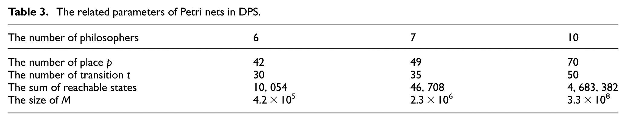
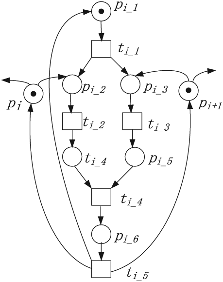
In Figure 14, p_i denotes the ith philosopher’s place when p_i_+ 1 represents the (i + 1)-th philosopher’s place and so on. For this experiment, 6, 7, and 10 philosophers are, respectively, chosen as the subject to be investigated. The related parameters of the chosen models are described in Table 3. The size of the state-space matrix M in a Petri net denotes the total number of elements in M.

Figure 14.

The fundamental unit of DPS.

Table 3.

The related parameters of Petri nets in DPS.

The number of philosophers	6	7	10
The number of place p	42	49	70
The number of transition t	30	35	50
The sum of reachable states	10, 054	46, 708	4, 683, 382
The size of M	4.2 × 10⁵	2.3 × 10⁶	3.3 × 10⁸

The evaluation index on algorithm performance

This article mainly focuses on the state-space reduction and state reachability, for which the state-space compression algorithm based on hybrid coding and the state reachability retrieval algorithm based on locally sensitive hashing are proposed. The evaluation indexes in compression and retrieval algorithm performance need to be considered for their assessment. For the compression algorithm, the compression ratio is an important evaluation index, reflecting the compression degree of the compression algorithm on the Petri net state space. The compression ratio CR is defined as follows

CR = \frac{B_{total}}{m \times n}

(14)

where m × n denotes the size of M before being compressed and B_total represents the size of the compressed state space.

For the proposed retrieval algorithm, the retrieval time is regarded as a critical evaluation index. The retrieval time RT is defined as follows

RT = t_{end} - t_{start}

(15)

where t_start and t_end, respectively, denote the time of submitting the query requirement and that of returning the query result. In most cases, many models need to be tested in a retrieval algorithm, leading to various experimental results. For a clearer analysis, the average retrieval time $\bar{RT}$ in equation (16) is also introduced as an evaluation index.

\bar{RT} = \frac{1}{k} \sum_{i = 1}^{k} R T_{i}

(16)

In equation (16), k and RT_i denote the number of retrieval and ith retrieval time, respectively. The average retrieval time can indicate the overall performance of the retrieval algorithms.

Experiment results and analysis

The experiment results of the state-space compression algorithm, compared with the RLE method under the same condition, are shown in Table 4.

Table 4.

The experiment result in the state-space compression algorithm.

Petri net models	m × n	B_total by the proposed algorithm	CR
Petri net models	m × n	B_total by the proposed algorithm	Our algorithm	RLE
Flexible manufacturing cell	26,750 × 26	276,436	39.75%	129.89%
6 dining philosophers’ system	10,054 × 42	87,953	20.83%	81.32%
7 dining philosophers’ system	46,708 × 49	460,005	20.10%	80.95%
10 dining philosophers’ system	4,683,382 × 70	60,174,928	18.36%	75.07%

Note: The bold value in table 4 shows the effective compression rate between the algorithm proposed in this paper and the RLE algorithm.

In Table 4, the proposed algorithm has better compression efficiency than the RLE. At best, the compression ratio of the proposed algorithm reaches 18.36%, which is about four times less than that in the RLE. Furthermore, the performance of the proposed algorithm manifests stability in multiple Petri net models. The RLE performs worst, with the compression ratio almost being 130% in the flexible manufacturing cell model.

Other experiment results of the state reachability retrieval are shown in Figure 15. Based on the location of the retrieved state in the state space, for convenient expression, four kinds of the retrieved states, namely, the initial state, the middle state, the final state, and the unreachable state are, respectively, labeled by numbers 1–4. The unreachable state is chosen by approximating the random reachable state. Meanwhile, the proposed state retrieval algorithm is compared with the linear search method. In consideration of the overall experimental performance of the retrieval algorithm, the average retrieval times based on four Petri net models are shown in Figure 16.

Figure 15.

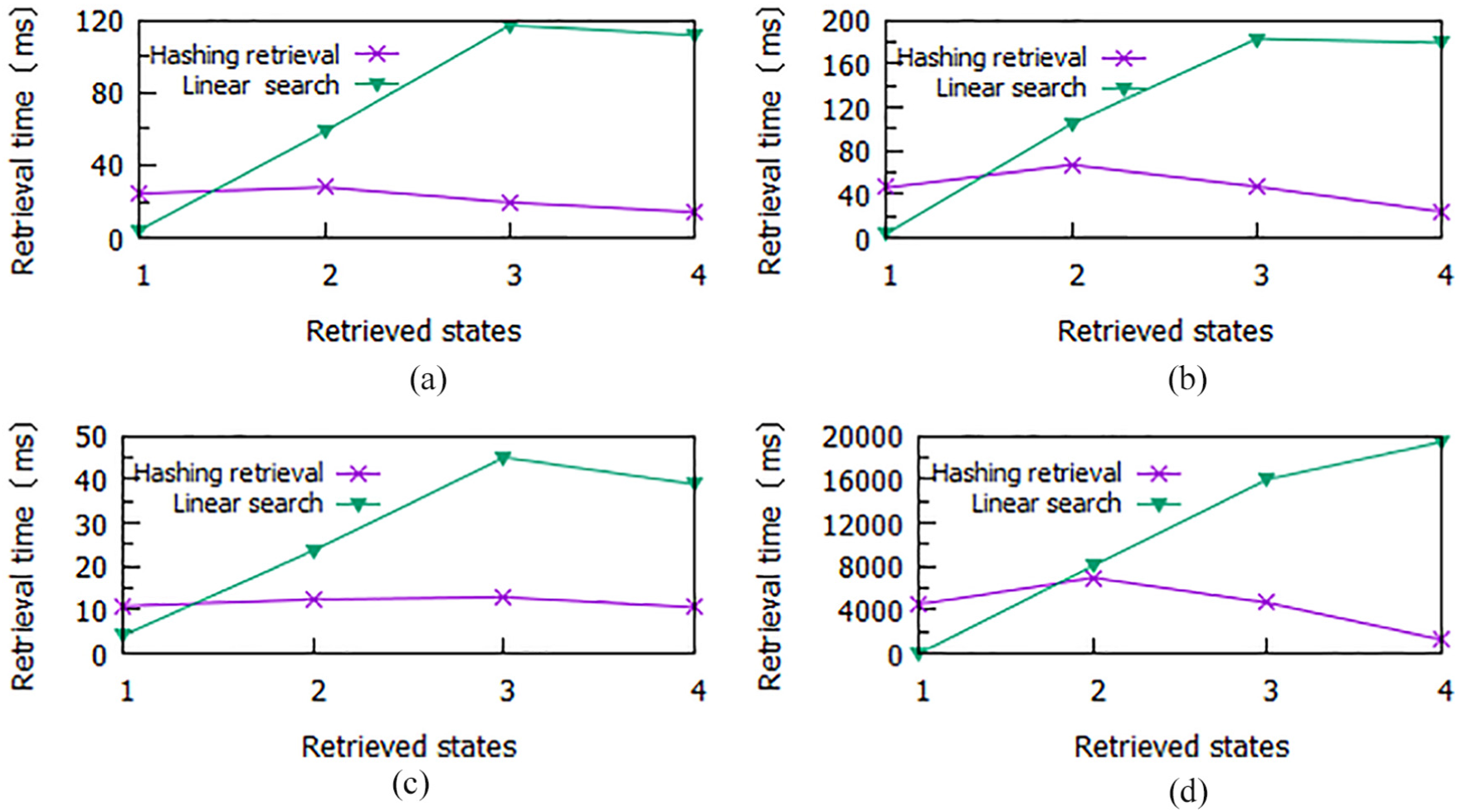
The experiment result in the state reachability retrieval algorithm. (a) Flexible manufacturing cell. (b) 6 dining philosophers’ system. (c) 7 dining philosophers’ system. (d) 10 dining philosophers’ systems.

Figure 16.

The average retrieval time versus various retrieved states.

Figures 15 and 16 show that the hashing retrieval algorithm proposed in this article has better time efficiency in the state retrieval, especially in the final state and the unreachable state. Compared with the traditional linear search method, the proposed algorithm possesses more robust adaptation over various state positions and Petri net models. The average time of the proposed algorithm is about 1/15 that of the linear search at best. The linear search method appears to be unstable, where the retrieval time increases linearly, making it unsuitable for massive data retrieval.

Note that the Petri net reduction techniques originally reported in Murata⁴⁰ can be used for state-space reduction, as did by Uzam.²⁸ In this article, we can use this method to simplify a plant model first if the reduction rules in Murata⁴⁰ are applicable. For example, the net shown in Figure 13 with 26 places can be reduced as shown in Figure 17. The reduced version with 23 places has 11,880 reachable states. Then, we can use the proposed state compression algorithms to compress its states. The estimated compression ratio will be calculated as 39.75% × (11,880/26,750) × (23/26) = 15.62%.

Figure 17.

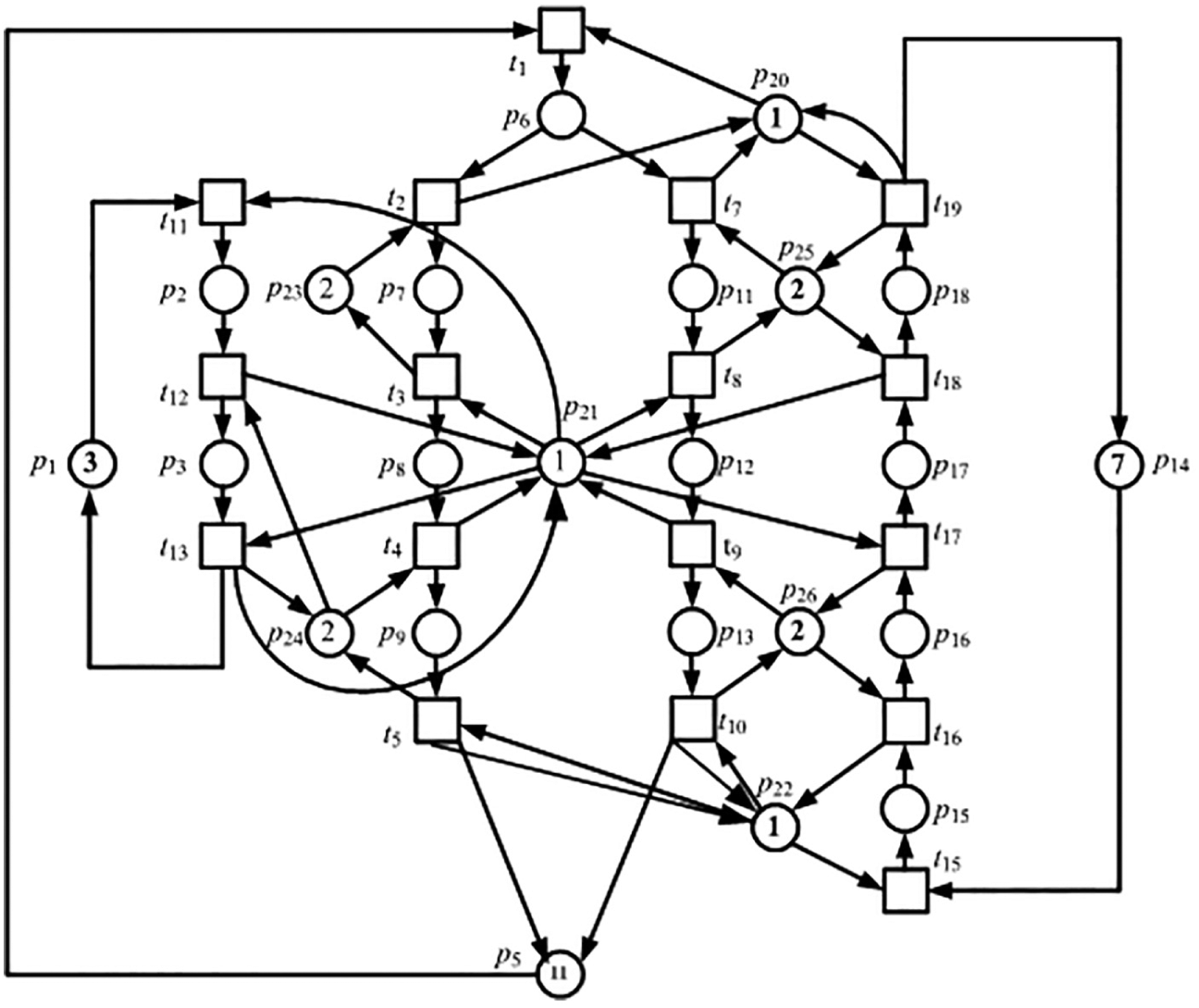
Reduced version of the Petri net model in Figure 13.

Conclusion

This article explores the relation between the state compression and the state retrieval and constructs a solution. For the reachability graph generation, the proposed caching arrangement algorithm of the reachability graph effectively solves the storage problem of the complete state space. Based on the data characteristic of the states in Petri nets, a hybrid coding algorithm is proposed to make a lossless compression for the states. Meanwhile, locally sensitive hashing is introduced to conduct a state retrieval on the compressed state space. The experiments show that the proposed algorithms achieve good performance in the state compression and state retrieval, offering a promising solution for relevant problems in Petri nets. Nevertheless, the compression efficiency in the proposed method is not ideal because of a balanced consideration on the state compression and the state reachability retrieval. At the same time, much time is spent in constructing the hashing index of the retrieval algorithm. In the future, we will explore more efficient compression algorithms by combining the other compression technique and investigate the retrieval algorithm that has a more concise index structure.

Footnotes

Handling Editor: ZhiWu Li

Declaration of conflicting interests

The author(s) declared no potential conflicts of interest with respect to the research, authorship, and/or publication of this article.

Funding

The author(s) disclosed receipt of the following financial support for the research, authorship, and/or publication of this article: This work is partially supported by the Fundamental Research Funds for the Central Universities with Grant Nos. K50510040013 and K5051304007 and the Doctoral Students’ Short-Term Study Abroad Scholarship Fund of Xidian University. The authors extend their appreciation to the Deanship of Scientific Research at King Saud University for funding this work through research group number RG-1439-005.

ORCID iD

Huorong Ren

References

Petri

CA.

Kommunikation mit Automaten. PhD Thesis, University of Bonn, Bonn, 1962.

Zhao

On controllability of dependent siphons for deadlock prevention in generalized Petri nets. IEEE T Syst Man Cy A 2008; 38: 369–384.

Chen

Barkaoui

et al . New Petri net structure and its application to optimal supervisory control: interval inhibitor arcs. IEEE T Syst Man Cy A 2014; 44: 1384–1400.

Chen

Barkaoui

et al . On the enforcement of a class of nonlinear constraints on Petri nets. Automatica 2015; 55: 116–124.

Viswanadham

Narahari

Johnson

TL.

Deadlock prevention and deadlock avoidance in flexible manufacturing systems using Petri net models. IEEE T Robotic Autom 1990; 6: 713–723.

Zhu

Bai

et al . Short-term scheduling of crude oil operations in refinery with high-fusion-point oil and two transportation pipelines. Enterp Inf Syst 2016; 10: 581–610.

Zhou

Elementary siphons of Petri nets and their application to deadlock prevention in flexible manufacturing systems. IEEE T Syst Man Cy A 2004; 34: 38–51.

Liu

You

et al . Fuzzy Petri nets for knowledge representation and reasoning: a literature review. Eng Appl Artif Intel 2017; 60: 45–56.

Yang

Qiao

et al . Scheduling of single-arm cluster tools for an atomic layer deposition process with residency time constraints. IEEE T Syst Man Cy: S 2017; 47: 502–516.

10.

Hou

Zhou

et al . Pareto-optimization for scheduling of crude oil operations in refinery via genetic algorithm. IEEE T Syst Man Cy: S 2017; 47: 517–530.

11.

Zhou

. Two-stage method for synthesizing liveness-enforcing supervisors for flexible manufacturing systems using Petri nets. IEEE Trans Indust Inform 2006; 2: 313–325.

12.

Wang

. Design of liveness-enforcing supervisors for flexible manufacturing systems using Petri nets. IEEE Trans Syst Man Cyber Part C 2007; 37: 517–526.

13.

Zhou

. Resource-oriented Petri net for deadlock avoidance in flexible assembly systems. IEEE Trans Syst Man Cyber Part A 2008; 38: 56–69.

14.

Zhou

. Control of elementary and dependent siphons in Petri nets and their application. IEEE Trans Syst Man Cybernet Part A 2008; 38: 133–148.

15.

Zhou

. A survey and comparison of petri net-based deadlock prevention policies for flexible manufacturing systems. IEEE Trans Syst Man Cybernet Part C 2008; 38: 173–188.

16.

Zhou

Jeng

. A maximally permissive deadlock prevention policy for fms based on Petri net siphon control and the theory of regions. IEEE Trans Automat Sci Eng 2008; 5: 182–188.

17.

Zhou

. Deadlock resolution in automated manufacturing systems: a novel Petri net approach. Berlin: Springer Science & Business Media, 2009.

18.

Wang

Wonham

WM.

Dynamic multiple-period reconfiguration of real-time scheduling based on timed DES supervisory control. IEEE T Ind Inform 2016; 12: 101–111.

19.

Hou

Barkaoui

Deadlock analysis and control based on Petri nets: a siphon approach review. Adv Mech Eng 2017; 9: 1–30.

20.

Silva

Valette

Petri nets and flexible manufacturing. In: European workshop on applications and theory in Petri nets, Bonn, 1 June 1989, pp.374–417. Heidelberg: Springer-Verlag.

21.

Silva

Teruel

A systems theory perspective of discrete event dynamic systems: the Petri net paradigm. In: Proceedings of the symposium discrete events manufacturing systems, 1996, pp.1–12. Berkeley, CA: CESA, http://webdiis.unizar.es/∼lrecalde/doctorado/bibliografia/CESA96.pdf

22.

Sadou

Demmou

Reliability analysis of discrete event dynamic systems with Petri nets. Reliab Eng Syst Safe 2009; 94: 1848–1861.

23.

Kim

A reliability analysis technique for object-oriented model using a reliability Petri net. Microelectron Reliab 1996; 36: 1237–1247.

24.

Cong

Fanti

Mangini

et al . Decentralized diagnosis by Petri nets and integer linear programming. IEEE T Syst Man Cy A 2018; 48: 1689–1700.

25.

Zhang

Feng

et al . Integration of learning-based testing and supervisory control for requirements conformance of black-box reactive systems. IEEE T Autom Sci Eng 2018; 15: 2–15.

26.

Zhang

Feng

ZW.

A learning-based synthesis approach to the supremal nonblocking supervisor of discrete-event systems. IEEE T Automat Contr Eng 2018; 63: 3345–3360.

27.

Zhu

et al . Fault identification of discrete event systems modeled by Petri nets with unobservable transitions. IEEE T Syst Man Cy A 2019; 49: 333–345.

28.

Liu

et al . Robust deadlock control for automated manufacturing systems with unreliable resources based on Petri net reachability graphs. IEEE T Syst Man Cy A. Epub ahead of print 23 April 2018. DOI: 10.1109/TSMC.2018.2815618

29.

Zhu

NQ.

Model-based fault identification of discrete event systems using partially observed Petri nets. Automatica 2018; 96: 201–212.

30.

Cong

Fanti

Mangini

AM.

On-line verification of current-state opacity by Petri nets and integer linear programming. Automatica 2018; 94: 205–213.

31.

et al . Improved multi-step look-ahead control policies for automated manufacturing systems. IEEE Access 2018; 6: 66824–66838.

32.

Wang

You

Seatzu

A novel approach for constraint transformation in Petri nets with uncontrollable transitions. IEEE T Syst Man Cy: S 2018; 48: 1403–1410.

33.

You

Wang

Dai

et al . An approach for enumerating minimal siphons in a subclass of Petri nets. IEEE Access 2018; 6: 4255–4265.

34.

Garg

An approach to performance specification of communication protocols using timed Petri nets. IEEE T Software Eng 1985; SE-11: 1216–1225.

35.

Uzam

The use of Petri net reduction approach for an optimal deadlock prevention policy for flexible manufacturing systems. Int J Adv Manuf Tech 2004; 23: 204–219.

36.

Liu

Hanisch

et al . Deadlock prevention based on structure reuse of Petri net supervisors for flexible manufacturing systems. IEEE T Syst Man Cy A 2012; 42: 178–191.

37.

Uzam

Gelen

et al . A divide-and-conquer-method for the synthesis of liveness enforcing supervisors for flexible manufacturing systems. J Intell Manuf 2016; 27: 1111–1129.

38.

Tong

Giua

On the equivalence of observation structures for Petri net generators. IEEE T Automat Contr 2016; 61: 2448–2462.

39.

Tong

Seatzu

et al . Verification of state-based opacity using Petri nets. IEEE T Automat Contr 2017; 62: 2823–2837.

40.

Giua

Design of optimal Petri net controllers for disjunctive generalized mutual exclusion constraints. IEEE T Automat Contr 2015; 60: 1774–1785.

41.

Giua

Decentralized supervision of Petri nets with a coordinator. IEEE T Syst Man Cy A 2015; 45: 955–966.

42.

Wang

Khemaissia

Khalgui

et al . Dynamic low-power reconfiguration of real-time systems with periodic and probabilistic tasks. IEEE T Autom Sci Eng 2015; 12: 258–271.

43.

Wang

ZW.

Synthesis of supervisory control with partial observation on normal state tree structures. IEEE T Autom Sci Eng. Epub ahead of print 28 December 2018. DOI: 10.1109/TASE.2018.2880178

44.

Giua

Characterization of admissible marking sets in Petri nets with conflicts and synchronizations. IEEE T Automat Contr 2017; 62: 1329–1341.

45.

Tong

et al . Basis marking representation of Petri net reachability spaces and its application to the reachability problem. IEEE T Automat Contr 2017; 62: 1078–1093.

46.

Valmari

The state explosion problem. In: Reisig

Rozenberg

(eds) Lectures on Petri nets I: basic models. Heidelberg: Springer-Verlag, 1996, pp.429–528.

47.

Murata

Petri nets: properties, analysis and applications. P IEEE 1989; 77: 541–580.

48.

Schmidt

Using Petri net invariants in state space construction. In: Garavel

Hatcliff

(eds) Tools and algorithms for the construction and analysis of systems. Heidelberg: Springer-Verlag, 2003, pp.473–488.

49.

Dragan

Leue

Alberto

LL.

Partial-order reduction for general state-exploring algorithms. Int J Softw Tools Te 2009; 11: 39–51.

50.

Piipponen

Valmari

Constructing minimal coverability sets. Fundam Inform 2016; 143: 393–414.

51.

Clarisó

Rodríguez-Carbonell

Cortadella

Derivation of non-structural invariants of Petri nets using abstract interpretation. In: Ciardo

Darondeau

(eds) Applications and theory of Petri nets. Heidelberg: Springer-Verlag, 2005, pp.188–207.

52.

Emerson

Wahl

Dynamic symmetry reduction. In: International conference on tools and algorithms for the construction and analysis of systems, Edinburgh, 4–8 April 2005, pp.382–396. Heidelberg: Springer-Verlag.

53.

Kurshan

Levin

Yenigün

Compressing transitions for model checking. In: International conference on computer aided verification, Copenhagen, 27–31 July 2002, pp.569–582. Heidelberg: Springer-Verlag.

54.

Bozga

Fernandez

Ghirvu

State space reduction based on live variables analysis. In: International static analysis symposium, Venice, 22–24 September 1999, pp.164–178. Heidelberg: Springer-Verlag.

55.

McMillan

KL.

Using unfoldings to avoid the state explosion problem in the verification of asynchronous circuits. In: International conference on computer aided verification, Montreal, QC, Canada, 29 June–1 July 1992, pp.164–177. Heidelberg: Springer-Verlag.

56.

Esparza

Römer

Vogler

An improvement of McMillan’s unfolding algorithm. Form Method Syst Des 2002; 20: 285–310.

57.

Fronk

Kehden

State space analysis of Petri nets with relation-algebraic method. J Symb Comput 2009; 44: 15–47.

58.

Reisig

Petri nets: an introduction. Heidelberg: Springer-Verlag, 2012.

59.

Miner

Ciardo

Efficient reachability set generation and storage using decision diagrams. In: International conference on application and theory of Petri nets, Williamsburg, VA, 21–25 June 1999, pp.6–25. Heidelberg: Springer-Verlag.

60.

Chen

ZW.

Optimal supervisory control of automated manufacturing systems. Boca Raton, FL: CRC Press, 2013.

61.

Bassiouni

MA.

Data compression in scientific and statistical databases. IEEE T Software Eng 1985; 10: 1047–1058.

62.

Asuquo

Nwachukwu

Ekong

NJ.

Application of run-length encoding technique in data Compression. J Appl Sci Res 2010; 6: 2123–2132.

63.

Memon

Adaptive coding of DCT coefficients by Golomb-Rice codes. In: International conference on image processing, Chicago, IL, 7 October 1998, pp.516–520. New York: IEEE.

64.

Basha

Jinaga

DB.

A robust image compression algorithm using JPEG 2000 standard with Golomb Rice coding. Int J Comput Sci Netw Secur 2010; 10: 26–33.

65.

Huang

Rao

RP.

Predictive coding. Wires Cogn Sci 2011; 2: 580–593.

66.

Kilner

Friston

Frith

CD.

Predictive coding: an account of the mirror neuron system. Cogn Process 2007; 8: 159–166.

67.

Mumolo

Francescato

Adaptive predictive coding of speech by means of Volterra predictors. In: IEEE winter workshop on nonlinear digital signal processing, Tampere, 17–20 January 1993, pp.2–4. New York: IEEE.

68.

Gionis

Indyk

Motwani

Similarity search in high dimensions via hashing. In: International conference on very large data bases, Edinburgh, 7–10 September 1999, pp.518–529. San Francisco, CA: Morgan Kaufmann.

69.

Koga

Ishibashi

Watanabe

Fast agglomerative hierarchical clustering algorithm using locality-sensitive hashing. Knowl Inf Syst 2007; 12: 25–53.

70.

Saad

Ahmad

Abu

et al . Hamming distance method with subjective and objective weights for personnel selection. Sci World J 2014; 2014: 865495.

71.

Ueno

Itoh

Utsunomiya

Adaptive predictive coding of still images using neural networks. Electron Commun Jpn 1993; 76: 31–41.

72.

Robinson

Cherry

Results of a prototype television bandwidth compression scheme. P IEEE 2005; 55: 356–364.

73.

Huang

Feng

Fang

Reverse query-aware locality-sensitive hashing for high-dimensional furthest neighbor search. In: IEEE international conference on data engineering, San Diego, CA, 19–22 April 2017, pp.167–170. New York: IEEE.

On state-space compression and state reachability retrieval of Petri nets

Abstract

Keywords

Introduction

Petri nets

Caching arrangement of the reachability graph algorithm

Basic methods on data compression and retrieval

The RLE

The Golomb–Rice coding

The adaptive prediction encoding

LSH

Hamming distance

State-space compression based on hybrid coding

Computation of local difference values

Encoding mode selection

The predictive value computation

RLE mode

State reachability retrieval based on locally sensitive hashing

Normalization of state length

Establishing the hash index structure

Primary state retrieval

Fine retrieval by returning

Experiment

Experiment models

The evaluation index on algorithm performance

Experiment results and analysis

Conclusion

Footnotes

Declaration of conflicting interests

Funding

ORCID iD

References