A new approach to the kinematic modeling of a three-dimensional car-like robot with differential drive using computational mechanics

Abstract

This article presents a kinematic analysis of a four-wheeled mobile robot in three-dimensions, introducing computational mechanics. The novelty lies in (1) the type of robot that is analyzed, which has been scarcely dealt with in the literature, and (2) the methodology used which enables the systematic implementation of kinematic algorithms using the computer. The mobile robot has four wheels, four rockers (like an All-Terrain Mobile Robot), and a main body. It also has two actuators and uses a drive mechanism known as differential drive (like those of a slip/skid mobile robot). We characterize the mobile robot as a set of kinematic closed chains with rotational pairs between links and a higher contact pair between the wheels and the terrain. Then, a set of generalized coordinates are chosen and the constraint equations are established. A new concept named “driving modes” has been introduced because some of the constraint equations are derived from these. The kinematics is the first step in solving the dynamics of this robot in order to set a control algorithm for an autonomous car-like robot. This methodology has been successfully applied to a real mobile robot, “Robotnik,” and the results are analyzed.

Introduction

A mobile robot involves advanced development in areas such as locomotion, sensing, navigation, and control. ¹ If wheels are used as the locomotion system, robots are known as wheeled mobile robots (WMRs), and in the world of WMRs, there are many wheel and axle configurations that have been used, which determine the kinematic properties of the robot. ² Campion et al. considered a general WMR with an arbitrary number of wheels of various types and various motorizations. They point out the structural properties of the kinematic models, taking into account the constraints on the robot’s mobility induced by the kinematic pairs. They also introduce the concepts of degree of mobility and degree of steerability and show the variety of possible robot constructions and wheel configurations.

Within WMRs, two broad families can be distinguished: (1) car-like four-WMRs (these can be referred to as OMRs or ordinary mobile robots), which are very popular because they are very easy to build, maintain, and control. Most of these robots can be analyzed in the x–y plane, that is, the robot’s motion can be considered in two dimensions (2D). (2) Articulated, all-terrain rovers (ATRs) with a sophisticated locomotion system, usually with six wheels and a suspension system, enable them to move on rough terrain. The motion is analyzed in three dimensions (3D). This type of robot has important applications such as deactivation of explosive devices, ³ space exploration missions, ⁴ and autonomous cars. ⁵

A subcategory of both OMRs and ATRs is made up of those that have differential kinematics: skid-steering mobile robots or SSMRs. ⁶ These usually have two, three, or four wheels.

The kinematic model of any kind of mobile robot is fundamental for navigation and control. The control system is in charge of managing the driving forces and their evolution over time to ensure correct navigation. Its objective is to connect different locations in space for the mobile robot by means of optimal trajectory planning. The process of calculating the driving forces involves solving the kinematics of the vehicle and their temporal evolution. That is why kinematics is so important, for which the mechanical structure and the locomotion system have to be considered.

Generally speaking, the modeling of the kinematics of OMRs can be classified, to date, into three main approaches: velocity vector, geometric, and transformation. ⁷ The velocity vector approach considers the velocity transformation between the robots’ rigid bodies, taking into account the local and global reference system. An example of this kind of analysis can be found in the work by Wang et al. ⁸ The geometric approach is based on the geometric relationships between the rigid bodies of the mobile robot. ⁹ With this approach, the relationship between the rigid body motion of the robot and the steering and drive rates of the wheels is developed. Explicit differential equations are derived to describe the rigid body motions. The transformation approach can be seen in the work by Muir and Neumann, ¹⁰ where matrix coordinate transformations and their derivatives are used to link the motion of the wheels to the motion of robots in a two-dimensional (2D) space, that is, translation in the x–y plane and yaw rotation. They also assume perfect rolling motion on a flat, smooth surface with no side or rolling slip. A recent paper based on this methodology applied to a 3D robot was the work by Tarokh and McDermott, ¹¹ where the authors use transformation matrices to obtain the kinematics of the Rocky 7 robot, a highly articulated prototype Mars rover. The kinematic model is then used to simulate the robot’s motion on different surfaces.

Other paper that uses a vectorial method to calculate velocities using matrix notation is the work by Seegmiller and Kelly. ¹² This paper presented a simple, algorithmic method to construct 3D kinematic models for WMR robots. Also, experimental results are presented to validate the model formulation, showing odometry improvement by calibrating to data logs and modeling 3D articulations. Kim and Lee ¹³ studied different robots’ working conditions to take advantage of the robot kinematics. In this paper, a kinematic-based rough terrain control has been developed to control the rover’s motion, keeping traction and minimizing energy consumption. The rover presents four-wheeled differential kinematics. The results of the experiments show good performance in terms of maximizing traction and minimizing energy use, while tracking the desired velocity despite traversing a variety of rough terrain types. A similar study on uneven terrains was done by Xu et al., ¹⁴ in a car-like robot with six independently driven wheels. Transformation matrix method is used to introduce the kinematics.

In any case, an important aspect to consider is the contact between the wheels and the ground. In the work by Ghotbi et al., ¹⁵ the interaction of the vehicle with different types of terrain has been analyzed.

One of the latest papers in which the kinematics is considered is the work by Zhang et al. ¹⁶ The authors analyzed what they call “the robot’s steering modes” in a multi-axle wheeled robot in order that the robot’s wheel can steer without slipping and it can improve its steering flexibility. Then, three steering control schemes are proposed. They have used an equivalent robot’s 2D model in their research.

In the work by Shuaiby et al., ¹⁷ a sliding mode–based robust tracking control for a redundant wheeled drive system is presented, which is designed for energy saving and fail safe motion. In this paper, the kinematics of the robot are obtained using a vectorial method expressed in a matricial way. Then, the four-WMRs are reduced at a 2D model. Simple dynamics properties are considered.

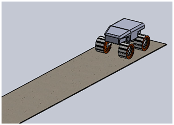
In this article, the direct kinematic problem has been solved for the mobile robot known as Robotnik (see Figure 1). This robot is a mixture of an OMR and an ATR, insofar as it consists of a main body, four wheels, four rocker arms, and a suspension system. It is an SSMR, four-wheeled differentially driven robot (OMR), but with four rocker arms (ATR), which normally moves on a generic road surface without longitudinal wheel slippage. Depending on what the authors call “driving modes,” the motion can be considered either in 2D (e.g. when it moves in a straight line on a horizontal road) or in 3D (e.g. when it travels over a bump).

Figure 1.

Robotnik robot to be modeled.

The chosen approach for analyzing the kinematics of this robot is different from the three types mentioned above. This new approach is based on computational mechanics. Two main novelties are introduced in this article: one is related to the type of robot analyzed and the other one with the method to solve it.

The Robotnik’s kinematics will be used, in future works, to calculate the dynamics and both the kinematics and dynamics will be used in control algorithms.

The mobile robot

The Robotnik robot to be modeled is as shown in Figure 1. It consists of the chassis, four rockers, and four fixed wheels (like an ATR) designed to move on surfaces that are not too steep (like an OMR). Without loss of generality, it is considered that the rear wheels are driven by two actuators. The rocker arms are attached to the chassis and wheels by means of revolution pairs of the same type R(y), that is, with the revolution axis in the local Y-direction (see Figure 3). Four torsion springs act on the rockers at the point where they join the chassis. There are also four dampers, the ends of which are attached to the chassis and the wheel (see Figure 2).

Figure 2.

Damper location.

This robot presents differential kinematics, that is, the wheels are fixed and only rotate around their center. Therefore, it can be considered an SSMR. In the contact between the tire and the ground, depending on the driving mode, there will be pure rolling and slip.

Kinematic analysis

We will solve the direct kinematic problem of the Robotnik robot when its geometry, the angular velocities of the rear wheels, and the driving mode are known. From the temporary values of the angles associated with the degrees of freedom (DOFs) of the system, the intention is to determine the position of all the system’s bars, as well as their velocities and accelerations. The results obtained will be used in future works to address the inverse dynamic problem, also known as the control problem, which involves calculating the driving forces. The resolution of the direct kinematic problem is necessary to solve the inverse dynamic problem, which in turn is fundamental for the control algorithm so that the robot can be autonomous.

Modeling the mobile robot

This robot has been modeled with nine bars, eight revolution pairs, and four contact pairs between the tire and the terrain. The revolution pairs are found in the joints between the rocker arms and the chassis and tires. They are of type R(y), that is, their rotational axes are aligned with the local Y-axis associated with the chassis.

The robot has $\mathit{F}=2\mathrm{DOFs}$ associated with the angles rotated by the rear wheels. Nevertheless, its motion takes place in 3D, since there is the possibility of yaw, pitch, and roll motions. Whether these types of motion occur will depend on the vehicle’s driving mode, which will be seen in section “Tire–ground contact pair.”

A robot configuration ${\mathit{C}}^j$ is uniquely established using ${\mathit{P}}_s=13$ significant points. Each significant point is defined by six variables (three Cartesian coordinates and three angles). The position and orientation in space of the significant point i are represented by the vector q as follows

$${\mathit{q}}_j^{\left\{i\right\}}=\{x_j^{\left\{i\right\}},y_j^{\left\{i\right\}},z_j^{\left\{i\right\}},{\phi }_j^{\left\{i\right\}},{\theta }_j^{\left\{i\right\}},{\psi }_j^{\left\{i\right\}}\}$$

where $i=1,\dots ,{\mathit{P}}_s$ is the point name and j is the configuration number. Any robot’s generic position is expressed as ${\mathit{q}}^{\{i\}}=\{x^{\{i\}},y^{\{i\}},z^{\{i\}},{\phi }^{\{i\}},{\theta }^{\{i\}},{\psi }^{\{i\}}\}$ .

These points are located at the center of mass (CM) of each bar. Two significant points are also used to characterize each tire–ground contact at $A,H,J,\mathrm{and}N$ . Their arrangement is shown in Figure 3. The tire–ground contact points for each wheel are shown in more detail in Figure 4.

Figure 3.

Location of the robot significant points.

Figure 4.

Significant points between the tire and the ground.

A generic configuration j can be expressed in terms of the significant points that define the robot, so that

$${\mathit{C}}^j={\mathit{C}}^j\left({\mathit{q}}_j^{\left\{i\right\}}\right)$$

where $i=1,\dots ,{\mathit{P}}_s$ .

Considering the elements of the vector ${\mathit{q}}_j^{\{i\}}$

$$\begin{array}{c}\multicolumn{1}{c}{{\mathit{C}}^j=\{x_j^{\left\{1\right\}},y_j^{\left\{1\right\}},z_j^{\left\{1\right\}},{\phi }_j^{\left\{1\right\}},{\theta }_j^{\left\{1\right\}},{\psi }_j^{\left\{1\right\}},x_j^{\left\{2\right\}},y_j^{\left\{2\right\}},z_j^{\left\{2\right\}},{\phi }_j^{\left\{2\right\}},}\\ {\theta }_j^{\left\{2\right\}},{\psi }_j^{\left\{2\right\}},\dots ,x_j^{\left\{13\right\}},y_j^{\left\{13\right\}},z_j^{\left\{13\right\}},{\phi }_j^{\left\{13\right\}},{\theta }_j^{\left\{13\right\}},{\psi }_j^{\left\{13\right\}}\}\hfill \end{array}$$

(1)

The variables used to define the configuration are not independent. In space, each free link has 6 DOFs, which implies the use of six variables to define its location and orientation. When connecting the bars to each other, depending on the type of kinematic pair, some of these DOFs are constrained. A 3D revolution pair has 1 DOF and five are constrained, which implies that five constraint conditions of the variables (constraint equations) must be introduced. For the connection between the tire and the ground, the treatment depends on the mobile robot’s driving mode. For example, if the vehicle moves in a straight line (moving with or without acceleration), it is considered that there is a pure rolling motion between the tire and the ground, which has 2 DOFs and introduces four constraint equations (see section “Tire–ground contact pair”). The total number P of significant points used in the modeling of the mobile robot is equal to the number of points ${\mathit{P}}_s$ used to define the geometry of the robot, plus the points required to characterize the tire–ground contact for each wheel ( $A,H,J,\mathrm{and}N$ , four points located on the ground, and the fixed bar, see Figure 3).

Therefore, $\mathit{P}={\mathit{P}}_s+4$ .

The total number of variables involved is

$$\mathit{N}=\mathit{P}\times 6=102$$

The DOFs of the mobile robot are

$$\mathit{F}=2\mathrm{GDL}$$

associated with rear wheel rotation. It is a sub-actuated vehicle, since the resulting motion can be 2D or 3D, depending on the “driving mode” concept introduced in section “Tire–ground contact pair.”

The number of constraint equations required is

$$\mathit{M}=\mathit{N}-\mathit{F}=100$$

(2)

Any generic configuration of the mobile robot is determined by the configuration vector ${\mathit{C}}^j$ given in equation (1), where the values of the variables are known.

Constraint equations

As stated in the previous section, the variables used to define a robot configuration are not independent. They are bound by the constraint equations. These equations are obtained from the following:

• Revolution pairs: giving rise to 40 equations;

• Contact points $\{A,H,J,N\}$ on the tires: 24 equations;

• Tire–ground contact for each wheel: 16 equations;

• Contact points $\{A,H,J,N\}$ on the ground: 16 equations;

• Considerations for chassis motion: 4 equations.

The resulting equations are analyzed in the following sections.

Revolution pair

Consider the revolution pair R in B, between rocker 2 and wheel 6 (Figure 5). This type of pair gives rise to the following constraint equations:

• 1. Vector equation 1: B is the common point of links 6 and 2; therefore

$$E{c}_1\equiv {}^0{\overrightarrow{r}}_{O_{0}B}={}^0{\overrightarrow{r}}_{O_0{O}_2}+{}^0{\overrightarrow{r}}_{O_{2}B}$$

(3)

where ${}^0{\overrightarrow{r}}_{O_{0}B}=\{x^{\{6\}},y^{\{6\}},z^{\{6\}}\}$ since ${\mathit{q}}^B=\{x^{\{6\}},y^{\{6\}},z^{\{6\}},{\phi }^{\{6\}},{\theta }^{\{6\}},{\psi }^{\{6\}}\}$ ; ${}^0{\overrightarrow{r}}_{O_0{O}_2}=\{x^{\{2\}},y^{\{2\}},z^{\{2\}}\}$ where ${\mathit{q}}^{O_2}=\{x^{\{2\}},y^{\{2\}},z^{\{2\}},{\phi }^{\{2\}},{\theta }^{\{2\}},{\psi }^{\{2\}}\}$ ; ${}^2{\overrightarrow{r}}_{O_{2}B}=\{-\frac{\mathrm{BC}}{2},0,0\}$ , where BC is the length of rocker 2.

$$\begin{array}{c}{}^0{\overrightarrow{r}}_{O_{2}B}=R_2^0·{}^2{\overrightarrow{r}}_{O_{2}B}\hfill \\ R_2^0=\mathrm{RotZ}\left({\phi }^{\left\{2\right\}}\right)·\mathrm{RotY}\left({\theta }^{\left\{2\right\}}\right)·\mathrm{RotX}\left({\psi }^{\left\{2\right\}}\right)\hfill \\ =\left(\begin{array}{ccc}\cos \left({\psi }^{\left\{2\right\}}\right)\cos \left({\theta }^{\left\{2\right\}}\right)\hfill & -\sin \left({\psi }^{\left\{2\right\}}\right)\cos \left({\theta }^{\left\{2\right\}}\right)+\cos \left({\psi }^{\left\{2\right\}}\right)\sin \left({\theta }^{\left\{2\right\}}\right)\cos \left({\phi }^{\left\{2\right\}}\right)\hfill & \sin \left({\psi }^{\left\{2\right\}}\right)\sin \left({\phi }^{\left\{2\right\}}\right)+\cos \left({\psi }^{\left\{2\right\}}\right)\sin \left({\theta }^{\left\{2\right\}}\right)\cos \left({\phi }^{\left\{2\right\}}\right)\hfill \\ \multicolumn{1}{c}{\sin \left({\psi }^{\left\{2\right\}}\right)\cos \left({\theta }^{\left\{2\right\}}\right)}& \cos \left({\psi }^{\left\{2\right\}}\right)\cos \left({\theta }^{\left\{2\right\}}\right)+\sin \left({\psi }^{\left\{2\right\}}\right)\sin \left({\theta }^{\left\{2\right\}}\right)\sin \left({\phi }^{\left\{2\right\}}\right)\hfill & -\cos \left({\psi }^{\left\{2\right\}}\right)\sin \left({\theta }^{\left\{2\right\}}\right)+\sin \left({\psi }^{\left\{2\right\}}\right)\sin \left({\theta }^{\left\{2\right\}}\right)\cos \left({\phi }^{\left\{2\right\}}\right)\hfill \\ \multicolumn{1}{c}{-\sin \left({\theta }^{\left\{2\right\}}\right)}& \cos \left({\theta }^{\left\{2\right\}}\right)\sin \left({\phi }^{\left\{2\right\}}\right)\hfill & \cos \left({\theta }^{\left\{2\right\}}\right)\cos \left({\phi }^{\left\{2\right\}}\right)\hfill \end{array}\right)\hfill \end{array}$$

• 2. Vector equation 2: the axis of rotation is common to links 6 and 2 (Figure 6)

$$E{c}_2\equiv {}^0{\overrightarrow{u}}_6\times {}^0{\overrightarrow{u}}_2=0\to R_6^0·{}^6{\overrightarrow{u}}_6\times R_2^0·{}^2{\overrightarrow{u}}_2=0$$

(4)

where ${}^2{\overrightarrow{u}}_2=\{0,1,0\}$ , ${}^6{\overrightarrow{u}}_6=\{0,1,0\}$

and

$$\begin{array}{c}\multicolumn{1}{c}{R_6^0=\mathrm{RotZ}\left({\phi }^{\left\{6\right\}}\right)·\mathrm{RotY}\left({\theta }^{\left\{6\right\}}\right)·\mathrm{RotX}\left({\psi }^{\left\{6\right\}}\right)}\\ =\left(\begin{array}{ccc}\cos \left({\psi }^{\left\{6\right\}}\right)\cos \left({\theta }^{\left\{6\right\}}\right)\hfill & -\sin \left({\psi }^{\left\{6\right\}}\right)\cos \left({\theta }^{\left\{6\right\}}\right)+\cos \left({\psi }^{\left\{6\right\}}\right)\sin \left({\theta }^{\left\{6\right\}}\right)\cos \left({\phi }^{\left\{6\right\}}\right)\hfill & \sin \left({\psi }^{\left\{6\right\}}\right)\sin \left({\phi }^{\left\{6\right\}}\right)+\cos \left({\psi }^{\left\{6\right\}}\right)\sin \left({\theta }^{\left\{6\right\}}\right)\cos \left({\phi }^{\left\{6\right\}}\right)\hfill \\ \multicolumn{1}{c}{\sin \left({\psi }^{\left\{6\right\}}\right)\cos \left({\theta }^{\left\{6\right\}}\right)}& \cos \left({\psi }^{\left\{6\right\}}\right)\cos \left({\theta }^{\left\{6\right\}}\right)+\sin \left({\psi }^{\left\{6\right\}}\right)\sin \left({\theta }^{\left\{6\right\}}\right)\sin \left({\phi }^{\left\{6\right\}}\right)\hfill & -\cos \left({\psi }^{\left\{6\right\}}\right)\sin \left({\theta }^{\left\{6\right\}}\right)+\sin \left({\psi }^{\left\{6\right\}}\right)\sin \left({\theta }^{\left\{6\right\}}\right)\cos \left({\phi }^{\left\{6\right\}}\right)\hfill \\ \multicolumn{1}{c}{-\sin \left({\theta }^{\left\{6\right\}}\right)}& \cos \left({\theta }^{\left\{6\right\}}\right)\sin \left({\phi }^{\left\{6\right\}}\right)\hfill & \cos \left({\theta }^{\left\{6\right\}}\right)\cos \left({\phi }^{\left\{6\right\}}\right)\hfill \end{array}\right)\hfill \end{array}$$

Figure 5.

Vectors used to model the revolution pair in B.

Figure 6.

Axle direction.

From the two previous vector equations, five scalar constraint equations are extracted. Operating and calling ${\mathbf{\Phi }}_i(\mathbf{q})$ the vector that contains the constraint equations, the equations are as follows

$$\begin{array}{c}{\mathbf{\Phi }}_1\left(\mathbf{q}\right)\equiv x^{\left\{2\right\}}-\frac{1}{2}·\cos \left({\psi }^{\left\{2\right\}}\right)\cos \left({\theta }^{\left\{6\right\}}\right)\mathrm{BC}-x^{\left\{6\right\}}\hfill \\ {\mathbf{\Phi }}_2\left(\mathbf{q}\right)\equiv y^{\left\{2\right\}}-\frac{1}{2}·\sin \left({\psi }^{\left\{2\right\}}\right)\cos \left({\theta }^{\left\{6\right\}}\right)\mathrm{BC}-y^{\left\{6\right\}}\hfill \\ {\mathbf{\Phi }}_3\left(\mathbf{q}\right)\equiv z^{\left\{2\right\}}+\frac{1}{2}·\sin \left({\theta }^{\left\{2\right\}}\right)\mathrm{BC}-x{z}^{\left\{6\right\}}\hfill \\ {\mathbf{\Phi }}_4\left(\mathbf{q}\right)\equiv \cos \left({\psi }^{\left\{2\right\}}\right)\cos \left({\theta }^{\left\{2\right\}}\right)+\sin \left({\psi }^{\left\{2\right\}}\right)\sin \left({\theta }^{\left\{2\right\}}\right)\sin \left({\phi }^{\left\{2\right\}}\right)\cos \left({\theta }^{\left\{6\right\}}\right)\sin \left({\phi }^{\left\{6\right\}}\right)\hfill \\ -\cos \left({\theta }^{\left\{2\right\}}\right)\sin \left({\phi }^{\left\{2\right\}}\right)\cos \left({\psi }^{\left\{6\right\}}\right)\cos \left({\phi }^{\left\{6\right\}}\right)+\sin \left({\psi }^{\left\{6\right\}}\right)\sin \left({\theta }^{\left\{6\right\}}\right)\sin \left({\phi }^{\left\{6\right\}}\right)\hfill \\ {\mathbf{\Phi }}_5\left(\mathbf{q}\right)\equiv \cos ({\theta }^{\left\{2\right\}})\cos \left({\phi }^{\left\{2\right\}}\right)·(\sin \left({\psi }^{\left\{6\right\}}\right)\cos \left({\phi }^{\left\{6\right\}}\right)+\cos \left({\psi }^{\left\{6\right\}}\right)\sin \left({\theta }^{\left\{6\right\}}\right)\sin \left({\phi }^{\left\{6\right\}}\right))\hfill \\ -(\sin \left({\psi }^{\left\{2\right\}}\right)\cos \left({\phi }^{\left\{2\right\}}\right)+\cos \left({\psi }^{\left\{2\right\}}\right)\sin \left({\theta }^{\left\{2\right\}}\right)\sin \left({\phi }^{\left\{2\right\}}\right))\cos \left({\theta }^{\left\{6\right\}}\right)\sin ({\phi }^{\left\{6\right\}})\hfill \end{array}$$

In all, there are 40 equations derived from the eight revolution pairs and they can be grouped in a single vector

$${\mathbf{\Phi }}_R\left(\mathbf{q}\right)=\left\{\begin{array}{c}\begin{array}{c}{\mathbf{\Phi }}_1\left(\mathbf{q}\right)\hfill \\ \multicolumn{1}{c}{{\mathbf{\Phi }}_2\left(\mathbf{q}\right)}\\ \multicolumn{1}{c}{{\mathbf{\Phi }}_3\left(\mathbf{q}\right)}\end{array}\hfill \\ \multicolumn{1}{c}{.}\\ \multicolumn{1}{c}{.}\\ \multicolumn{1}{c}{.}\\ \multicolumn{1}{c}{.}\\ \multicolumn{1}{c}{{\mathbf{\Phi }}_{40}\left(q\right)}\end{array}\right\}$$

(5)

Tire–ground contact pair

To characterize this contact pair, it is necessary to distinguish two different aspects: on the one hand, the type of wheel used, and on the other hand, the “driving modes” of the mobile robot. In this robot, the wheels are conventional. The mobile robot’s so-called “driving modes” are related to the characteristics of its motion according to three criteria:

1. Type of surface on which it moves;

2. Trajectory followed;

3. Type of motion.

According to the above criteria, the driving modes are as follows:

Type of surface	Trajectory	Motion
a. Smooth flat surface (horizontal or sloping)	a.1 Straight: a.1.1 X = cte a.1.2 Y = cte a.1.3 bX + cY = cte	a.1.i.1 With positive acceleration (traction), i = 1…3
		a.1.i.2 With constant vel.
		a.1.i.3 With negative acceleration (braking)
	a.2 Curve: F(X, Y) = 0	a.2.1 With positive acceleration (traction)
		a.2.2 With constant vel.
		a.2.3 With negative acceleration (braking)
b. Smooth curved surface	b.1 Straight: b.1.1 Z = F(X = cte, Y) b.1.2 Z = F(X, Y = cte) b.1.3 Z = F(aX + bY = cte)	b.1.i.1 With positive acceleration (traction), i = 1,…,3
		b.1.i.2 With constant vel.
		b.1.i.3 With negative acceleration (braking)
	b.2 Curve: Z = F(X, Y)	b.2.1 With positive acceleration (traction)
		b.2.2 With constant vel.
		b.2.3 With negative acceleration (braking)
c. Flat rough and/or uneven surface (horizontal or sloping)
d. Rough and/or irregular curved surface

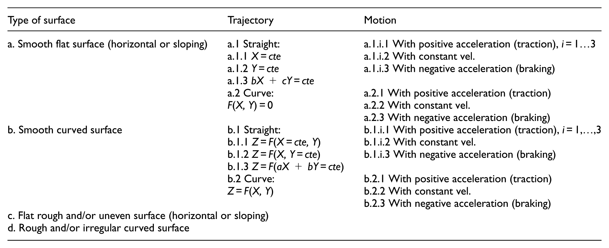
To characterize the tire–ground contact pair, it is necessary to consider that the mobile robot presents differential kinematics, that is, the wheels of the mobile robot are of the fixed type. This means that they have a fixed angle with respect to the chassis of the vehicle, and they are forced to move forward or backward in the plane that contains the wheel and can only rotate around their axis.

On the other hand, each “driving mode” has certain peculiarities that must be reflected in the constraint equations. For example, for the driving mode “a.2.2” (curves on a flat horizontal surface at a constant speed), it must be considered that the inner wheels must rotate slower than the outer wheels for the vehicle to describe the curve (Figure 7).

Figure 7.

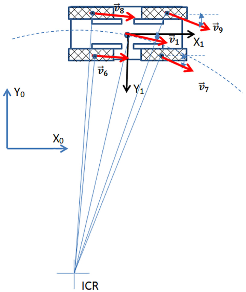
The vehicle as a whole, as a solid rigid body, follows a circular path around the ICR (instant center of rotation).

Let us analyze “driving mode” a.1.1.2 (driving in a straight line on a flat surface at a constant speed) in more detail. In the contact between the tire and the ground, there is a rolling pair, and it is assumed that there is no sliding in the longitudinal direction of the motion X. The wheel is allowed to make turns around the X-, Y-, and Z-axes, although the rotation about the Y-axis is related to its longitudinal displacement X. For link number 6 (wheel) and contact point A, see Figure 8.

Figure 8.

Rolling pair at the tire–ground contact point.

The constraint equations are as follows

$$E{c}_3\equiv {}^0{\overrightarrow{r}}_{O_0{A}_6}={}^0{\overrightarrow{r}}_{O_0{A}_1}$$

(6)

Developing equation (6) and considering that point $A_6$ belongs to link 6 then

$${}^0{\overrightarrow{r}}_{O_0{A}_6}={}^0{\overrightarrow{r}}_{O_{0}B}+{}^0{\overrightarrow{r}}_{{\mathrm{BA}}_6}$$

(7)

The contact point is a common point. It cannot be detached from the ground or embedded in it

$$E{c}_4\equiv x^{\left\{i\right\}}=R·{\theta }^{\left\{i\right\}}$$

(8)

The angle of rotation about the Y-axis is related to the longitudinal displacement of the wheel axis. Equation (6) can be expressed as follows.

Following the numeration from equation (5), the new constraint equations are

$$\begin{array}{c}{\mathbf{\Phi }}_{41}\left(\mathbf{q}\right)\equiv x^{\left\{14\right\}}-x^{\left\{10\right\}}\hfill \\ {\mathbf{\Phi }}_{42}\left(\mathbf{q}\right)\equiv y^{\left\{14\right\}}-y^{\left\{10\right\}}\hfill \\ {\mathbf{\Phi }}_{43}\left(\mathbf{q}\right)\equiv z^{\left\{14\right\}}-z^{\left\{10\right\}}\hfill \\ {\mathbf{\Phi }}_{44}\left(\mathbf{q}\right)\equiv x^{\left\{6\right\}}=R·{\theta }^{\left\{6\right\}}\hfill \end{array}$$

Considering the four contact points, 16 new equations are introduced. And, from equation (7), because the contact point A (10) is related to link 6

$$\begin{array}{c}{\mathbf{\Phi }}_{45}\left(\mathbf{q}\right)\equiv x^{\left\{6\right\}}-(\sin \left({\psi }^{\left\{6\right\}}\right)·\cos \left({\phi }^{\left\{6\right\}}\right)+\cos \left({\psi }^{\left\{6\right\}}\right)·\cos \left({\theta }^{\left\{6\right\}}\right)·\sin \left({\theta }^{\left\{6\right\}}\right))·R-x^{\left\{10\right\}}\hfill \\ {\mathbf{\Phi }}_{46}\left(\mathbf{q}\right)\equiv y^{\left\{6\right\}}-(-\cos \left({\psi }^{\left\{6\right\}}\right)·\sin \left({\phi }^{\left\{6\right\}}\right)+\sin \left({\psi }^{\left\{6\right\}}\right)·\cos \left({\theta }^{\left\{6\right\}}\right)·\sin \left({\theta }^{\left\{6\right\}}\right))·R-y^{\left\{10\right\}}\hfill \\ {\mathbf{\Phi }}_{47}\left(\mathbf{q}\right)\equiv z^{\left\{6\right\}}-\cos \left({\theta }^{\left\{6\right\}}\right)·\cos \left({\phi }^{\left\{6\right\}}\right)·R-z^{\left\{10\right\}}\hfill \\ {\mathbf{\Phi }}_{48}\left(\mathbf{q}\right)\equiv {\psi }^{\left\{6\right\}}-{\psi }^{\left\{10\right\}}\hfill \\ {\mathbf{\Phi }}_{49}\left(\mathbf{q}\right)\equiv {\phi }^{\left\{6\right\}}-{\phi }^{\left\{10\right\}}\hfill \\ {\mathbf{\Phi }}_{50}\left(\mathbf{q}\right)\equiv {\theta }^{\left\{6\right\}}-{\theta }^{\left\{10\right\}}\hfill \end{array}$$

In addition, 24 more equations are generated by considering the other three contact points. At this stage, 40 new equations have been introduced. In all, up to know there are 80 equations.

Considerations for the movement of link 1 (chassis) according to the driving mode

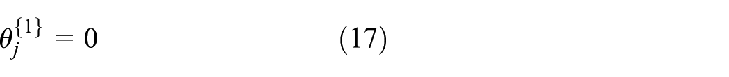
Several considerations must be taken into account when modeling the actual behavior of the vehicle in motion. On the one hand, when the vehicle moves on a flat surface in a straight line at a constant velocity, there are no rolling, pitching, or yawing angles. On the other hand, the height of the CM remains constant. Therefore, the following additional constraint equations must be considered

$$\begin{array}{c}{z}_j^{\left\{1\right\}}=K;\mathrm{for}\mathrm{a}\mathrm{horizontal}\mathrm{flat}\mathrm{surface},\hfill \\ K=h,\mathrm{i}.\mathrm{e}.\mathrm{the}\mathrm{height}\mathrm{of}\mathrm{the}\mathrm{CM}\mathrm{for}\mathrm{rod}1\hfill \end{array}$$

(9)

$${\phi }_j^{\left\{1\right\}}=0$$

(10)

$${\theta }_j^{\left\{1\right\}}=0$$

(11)

$${\psi }_j^{\left\{1\right\}}=0$$

(12)

When the vehicle describes a curved path at a constant speed on a flat horizontal surface, the outer wheels rotate faster than the inner wheels and a normal acceleration is generated that influences the vehicle roll angle. In addition, the position of the CM changes and the steering angle must take certain values so that the vehicle describes the curve correctly

$$x_j^{\left\{1\right\}}=P_1+R_c·\sin (-{\phi }^{\left\{1\right\}})+z^{\left\{1\right\}}\sin \left({\psi }^{\left\{1\right\}}\right)·\sin (-{\phi }^{\left\{1\right\}})$$

(13)

$$y_j^{\left\{1\right\}}=R_c·\cos (-{\phi }^{\left\{1\right\}})-R_c+z^{\left\{1\right\}}\sin \left({\psi }^{\left\{1\right\}}\right)·\cos (-{\phi }^{\left\{1\right\}})$$

(14)

$$z_j^{\left\{1\right\}}=h·\cos \left({\psi }^{\left\{1\right\}}\right)$$

(15)

$${\psi }_j^{\left\{1\right\}}=K_{\mathrm{Bal}}·\frac{{(-{\stackrel{·}{\theta }}^{\left\{6\right\}}·R)}^2}{R_c}$$

(16)

$${\theta }_j^{\left\{1\right\}}=0$$

(17)

$${\phi }_j^{\left\{1\right\}}=\frac{-{\theta }^{\left\{6\right\}}·R}{R_c·(1-a/2·\mathrm{Rc})}$$

(18)

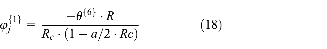
where j = 1 … is the number of configurations, R is the radius of the tire, $R_c$ is the radius of the curve, a is the distance between the wheels, $K_{\mathrm{Bal}}$ is the roll stiffness, and $P_1$ is the initial position of the vehicle in X.

When the vehicle accelerates or brakes, a transfer of load occurs in the vehicle that affects the pitch angle. The height of the CM also changes. These characteristics must also be present in the constraint equations. Liu et al. ¹⁸ studied the reliability on a car’s brake system.

Additional constraint equations

The contact points $\{A,H,J,N\}$ are part of the ground which leads to four more constraint equations

$$z_j^{\left\{14\right\}}=K_1$$

(19)

$$z_j^{\left\{15\right\}}=K_2$$

(20)

$$z_j^{\left\{16\right\}}=K_3$$

(21)

$$z_j^{\left\{17\right\}}=K_4$$

(22)

where the constant $K_i$ with $(i=1,\dots ,4)$ depends on the type of surface and j is the configuration number. For horizontal surfaces, $K_i=0$ .

Since the contact points with the ground do not spin $\{{\phi }_j^{\{17\}},{\theta }_j^{\{17\}},{\psi }_j^{\{17\}}\}$ , the following equations can be added for each point such as equation (17)

$${\phi }_j^{\left\{17\right\}}=0$$

(23)

$${\theta }_j^{\left\{17\right\}}=0$$

(24)

$${\psi }_j^{\left\{17\right\}}=0$$

(25)

It leads to 12 additional equations. Finally, the set of constraint equations (considering all revolution pairs and the contact points of the tire with the ground, and taking into account the different driving styles) leads to a 100 × 102 system of equations ( M  = 100).

All the constraints can be grouped in a single vector

$$\mathbf{\Phi }\left(\mathbf{q}\right)=\left\{\begin{array}{c}\begin{array}{c}{\mathbf{\Phi }}_1\left(\mathbf{q}\right)\hfill \\ \multicolumn{1}{c}{{\mathbf{\Phi }}_2\left(\mathbf{q}\right)}\\ \multicolumn{1}{c}{{\mathbf{\Phi }}_3\left(\mathbf{q}\right)}\end{array}\hfill \\ \multicolumn{1}{c}{.}\\ \multicolumn{1}{c}{.}\\ \multicolumn{1}{c}{.}\\ \multicolumn{1}{c}{.}\\ \multicolumn{1}{c}{{\mathbf{\Phi }}_{100}\left(q\right)}\end{array}\right\}$$

(26)

Resolution of the constraint equations

Position problem

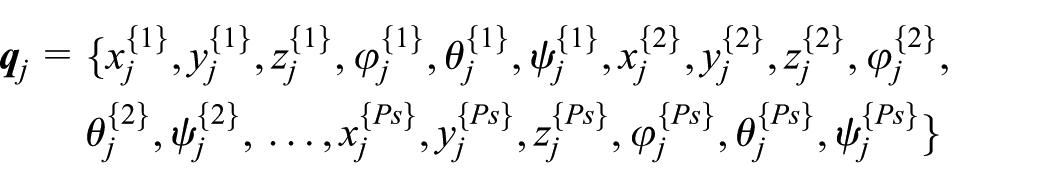
The coordinate vector of the vehicle defining a j-configuration of the mobile robot is as follows

$$\begin{array}{c}\multicolumn{1}{c}{{\mathit{q}}_j=\{x_j^{\left\{1\right\}},y_j^{\left\{1\right\}},z_j^{\left\{1\right\}},{\phi }_j^{\left\{1\right\}},{\theta }_j^{\left\{1\right\}},{\psi }_j^{\left\{1\right\}},x_j^{\left\{2\right\}},y_j^{\left\{2\right\}},z_j^{\left\{2\right\}},{\phi }_j^{\left\{2\right\}},}\\ {\theta }_j^{\left\{2\right\}},{\psi }_j^{\left\{2\right\}},\dots ,x_j^{\left\{\mathrm{Ps}\right\}},y_j^{\left\{\mathrm{Ps}\right\}},z_j^{\left\{\mathrm{Ps}\right\}},{\phi }_j^{\left\{\mathrm{Ps}\right\}},{\theta }_j^{\left\{\mathrm{Ps}\right\}},{\psi }_j^{\left\{\mathrm{Ps}\right\}}\}\hfill \end{array}$$

where ${\mathit{P}}_s=17$ .

The position problem consists of calculating the variables of the coordinate vector from the DOF of the mobile robot. These coordinates are bounded by the M constraint equations, which are grouped in the constraint vector $\mathbf{\Phi }$ .

The solution of the system of constraint equations provides the desired values

$$\mathbf{\Phi }\left(\mathbf{q}\right)=0$$

(27)

This is a non-linear equation system, which can be solved using Newton’s method. For this purpose, it is necessary to estimate the variables for a certain configuration of the mobile robot

$$\begin{array}{c}\multicolumn{1}{c}{{\mathit{q}}^0=\{x_1^0,y_1^0,z_1^0,{\phi }_1^0,{\theta }_1^0,{\psi }_1^0,x_2^0,y_2^0,z_2^0,{\phi }_2^0,{\theta }_2^0,{\psi }_2^0,\dots ,x_{13}^0,}\\ y_{13}^0,z_{13}^0,{\phi }_{13}^0,{\theta }_{13}^0,{\psi }_{13}^0\}\hfill \end{array}$$

(28)

Equation (28), using the Taylor series, can be rewritten as follows

$${\mathbf{\Phi }}_q\left({\mathit{q}}_i\right)·({\mathit{q}}_{i+1}-{\mathit{q}}_i)=-\mathbf{\Phi }\left({\mathit{q}}_i\right)$$

(29)

The matrix ${\mathbf{\Phi }}_{\mathit{q}}$ of the equation system as given by equation (5) is the Jacobian. Each row contains the first-order partial derivatives of the corresponding constraint equation with respect to each of the coordinates. Its dimensions are M × N (M = 100 and N = 102)

$${\left(\begin{array}{ccc}\frac{\partial {\mathbf{\Phi }}_1}{\partial {\mathit{q}}_j^1}\hfill & \cdots \hfill & \frac{\partial {\mathbf{\Phi }}_1}{\partial {\mathit{q}}_j^N}\hfill \\ \multicolumn{1}{c}{⋮}& \ddots \hfill & ⋮\hfill \\ \multicolumn{1}{c}{\frac{\partial {\mathbf{\Phi }}_M}{\partial {\mathit{q}}_j^1}}& \cdots \hfill & \frac{\partial {\mathbf{\Phi }}_M}{\partial {\mathit{q}}_j^N}\hfill \end{array}\right)}_{\mathit{M}\times \mathit{N}}$$

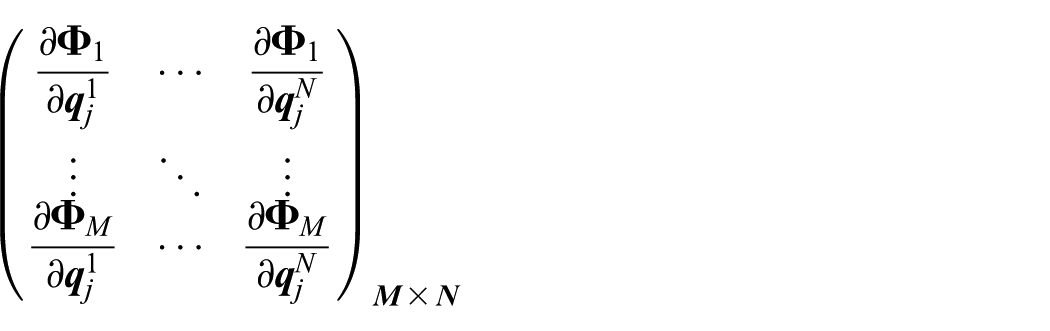
Note that the variables associated with the DOF are known and in successive iterations they take the same value and can be eliminated together with the corresponding columns of the Jacobian.

The system of non-linear equation (30) becomes a system with dimensions $\mathit{M}\times \mathit{M}$ . Once the position problem is solved, the configuration of the mobile robot is determined for each DOF

$$\begin{array}{c}\multicolumn{1}{c}{{\mathit{q}}_j=\{x_j^{\left\{1\right\}},y_j^{\left\{1\right\}},z_j^{\left\{1\right\}},{\phi }_j^{\left\{1\right\}},{\theta }_j^{\left\{1\right\}},{\psi }_j^{\left\{1\right\}},x_j^{\left\{2\right\}},y_j^{\left\{2\right\}},z_j^{\left\{2\right\}},{\phi }_j^{\left\{2\right\}},}\\ {\theta }_j^{\left\{2\right\}},{\psi }_j^{\left\{2\right\}},\dots ,x_j^{\left\{\mathrm{Ps}\right\}},y_j^{\left\{\mathrm{Ps}\right\}},z_j^{\left\{\mathrm{Ps}\right\}},{\phi }_j^{\left\{\mathrm{Ps}\right\}},{\theta }_j^{\left\{\mathrm{Ps}\right\}},{\psi }_j^{\left\{\mathrm{Ps}\right\}}\}\hfill \end{array}$$

The vector ${\mathit{q}}_j$ is known for $j=1,\dots ,N_c$ , where $N_c$ is the number of configurations for which the value of the variables associated with the DOF is known.

Velocity problem

The velocity problem consists of solving the temporal derivatives of the coordinates of the mechanical system. Briefly, the constraint equations are

$$\mathbf{\Phi }\left(\mathbf{q}\right)=0$$

Deriving the above expression with respect to time

$${\mathbf{\Phi }}_{\mathit{q}}\left(\mathit{q}\right)·\stackrel{·}{\mathit{q}}=0$$

(30)

The system of equation (5) is linear, where the unknowns are the elements of the vector of velocities $\stackrel{·}{\mathit{q}}$ . The Jacobian matrix is known from the previous section. It consists of M equations (100) and N variables (102). The velocities associated with the DOF are known and can be passed to the second term of the equation, leading to a square system where $\mathit{M}=100$ .

Acceleration problem

The acceleration problem consists of solving the temporal derivatives of the velocities.

Deriving equation (5) with respect to time

$${\mathbf{\Phi }}_{\mathit{q}}\left(\mathit{q}\right)·\stackrel{··}{\mathit{q}}=-{\stackrel{·}{\mathbf{\Phi }}}_{\mathit{q}}·\stackrel{·}{\mathit{q}}$$

(31)

Both the Jacobian matrix and the right term of the equation, which is a function of the positions and velocities, are known. This leads to a linear system of $\mathit{M}=100$ equations with $\mathit{N}=102$ variables. The accelerations associated with the DOF of the system are known, so by performing the relevant operations, the previous system is reduced to a square where $\mathit{M}=100$ . The unknowns are the elements of the vector of accelerations $\stackrel{··}{\mathit{q}}$ .

Transition from a straight line to a circumference arc: the clothoid curve

When a mobile robot moves in a straight line, there is no normal acceleration. However, when it turns (e.g. following an arc), there is a normal acceleration

$$a_n=\frac{v^2}{R}$$

(32)

where v is the vehicle’s velocity and R is the radius of curvature.

If the vehicle moves in a straight line and approaches a curve, at the point of tangency, it experiences a sudden change in the centrifugal acceleration (as well as in the radius of curvature and the curve itself). The same occurs when the vehicle exits the circular curve.

In order to achieve a progressive change in the value of the normal acceleration (and all other parameters), a transition curve must be introduced between the straight line and the circular arc. Since the velocity of the vehicle is intended to be constant at any position, whether straight or curved, the element must allow a variation in the radius. A desirable situation is to achieve a constant, progressive, uniform, linear variation of the normal acceleration (Figure 9).

Figure 9.

Link between a straight section and a circular section with the clothoid curve.

If the link between the straight line and the curve of radius R is performed by a transition curve of length $l_c$ and the centrifugal acceleration is intended to change from 0 to $v^2/R_c$ , an acceleration per unit of length is required

$$a_{\mathrm{nu}}=\frac{\frac{v^2}{R_c}}{l_c}$$

(33)

If the transition curve changes its radius from $\infty$ in the straight line to $R_c$ in the circular curve, for a generic point of the curve located at a distance l from the beginning of the curve, the mobile robot in contact with the straight line will undergo a centrifugal acceleration. It can be expressed in terms of the unit normal acceleration, as follows

$$a_n=\frac{\frac{v^2}{R_c}}{l_c}l$$

(34)

In addition

$$a_n=\frac{v^2}{R}$$

(35)

Matching both equations

$$\frac{v^2}{R}=\frac{\frac{v^2}{R_c}}{l_c}l=\frac{v^2·l}{R_c·l_c}$$

(36)

As a result, equation (35) can be rewritten as follows: $R_c·l_c=R·l$ .

And replacing this, $R_c·l_c=K^2$ . The equation defining the clothoid curve is $R·l=K^2$ , which is a transition curve between a straight section and a circular path so that the normal acceleration undergone by the vehicle is progressive rather than abrupt.

Examples of resolution of the direct kinematics of the mobile robot

It is worthwhile to note that the computational time needed to obtain a solution (motion simulation following a desired path) is just a few milliseconds for the proposed examples. The direct kinematics are solved for the following four simple cases.

Case A: driving in a straight line on a flat surface at a constant velocity

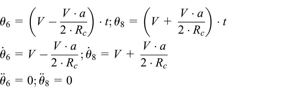
The vehicle moves in a straight line in the X-direction. Since it is a differential drive vehicle, the angular velocity of each rear wheel is the same (Figure 10). The values of the independent coordinates associated with the rotation of the rear wheels (6 and 8), angular velocities, and angular accelerations are as follows (Figure 11)

$$\begin{array}{c}{\theta }_6=K·t;{\theta }_8=K·t\hfill \\ {\stackrel{·}{\theta }}_6=K;{\stackrel{·}{\theta }}_8=K\hfill \\ {\stackrel{··}{\theta }}_6=0;{\stackrel{··}{\theta }}_8=0\hfill \end{array}$$

Figure 10.

Mobile robot moving in a straight line on a horizontal surface.

Figure 11.

Kinematics for case A.

The values of the rotated angle, angular velocity, and angular acceleration of the wheels are shown in graphs a1, a2, and a3), respectively, for a value of K = 6. The rotated angle varies linearly, with constant angular velocity and zero angular acceleration.

The results of position, velocity, and acceleration for rod 1 of the vehicle are shown in graphs a4, a5, and a6). As expected, they show how the longitudinal displacement increases linearly. The transverse displacement takes a constant value, since the vehicle moves in a straight line parallel to the X-axis. The longitudinal linear velocity is constant and the linear acceleration is zero.

Case B: driving in a straight line on a flat surface with constant acceleration

The values of the independent coordinates associated with the rotation of the rear wheels (6 and 8), angular velocities, and angular accelerations are as follows (Figure 12)

$$\begin{array}{c}{\theta }_6=K·t^2;{\theta }_8=K·t^2\hfill \\ {\stackrel{·}{\theta }}_6=2·K·t;{\stackrel{·}{\theta }}_8=2·K·t\hfill \\ {\stackrel{··}{\theta }}_6=2·K;{\stackrel{··}{\theta }}_8=2·K\hfill \end{array}$$

Figure 12.

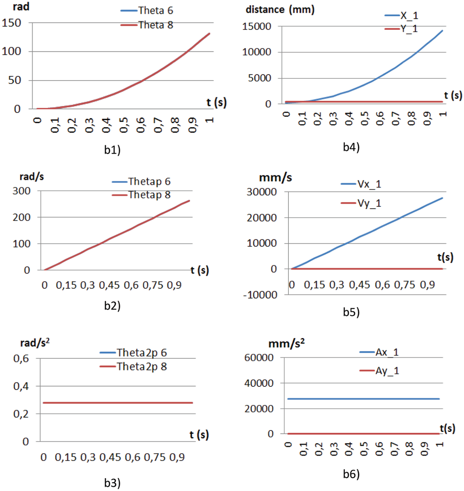
Kinematics for case B.

The value of K is defined as 0.14. Graph b4 shows that the distance traveled by the vehicle is not linear, as the angle rotated by the wheels is not linear. The velocity of rod 1 is linear, as is the angular velocity of the wheels (b2). The acceleration of the vehicle is constant in the X-direction and 0 in the transverse direction, since the vehicle moves in a straight line in the X-direction (see b6).

Case C: driving in a circular curve on a flat surface at a constant velocity

The values of the independent coordinates associated with the rotation of the rear wheels (6 and 8), angular velocities, and angular accelerations are as follows (Figures 13 and 14)

$$\begin{array}{c}{\theta }_6=(V-\frac{V·a}{2·R_c})·t;{\theta }_8=(V+\frac{V·a}{2·R_c})·t\hfill \\ {\stackrel{·}{\theta }}_6=V-\frac{V·a}{2·R_c};{\stackrel{·}{\theta }}_8=V+\frac{V·a}{2·R_c}\hfill \\ {\stackrel{··}{\theta }}_6=0;{\stackrel{··}{\theta }}_8=0\hfill \end{array}$$

Figure 13.

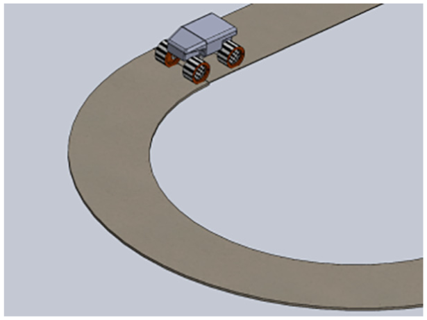
Mobile robot describing a circular line on a horizontal surface.

Figure 14.

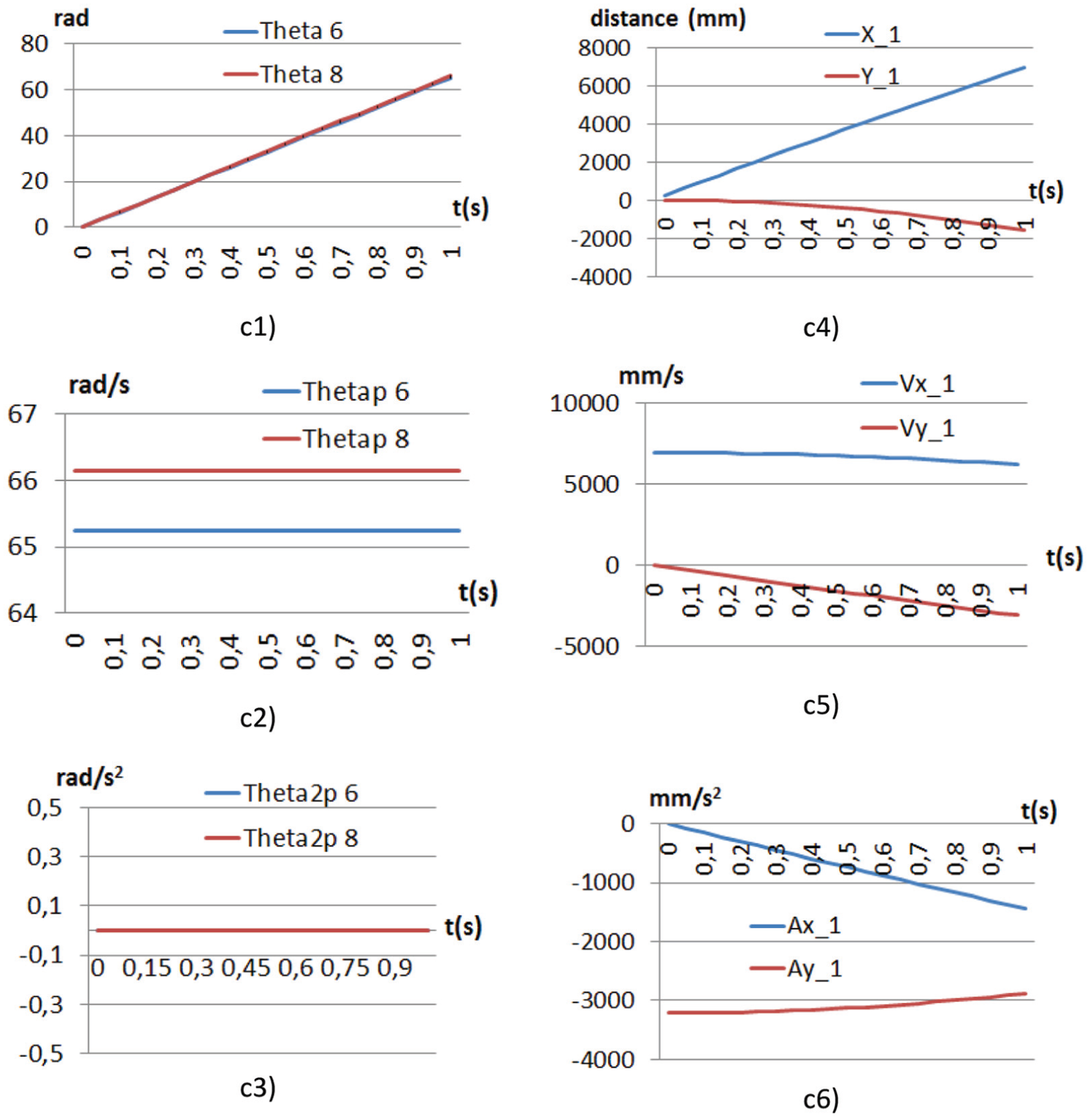
Kinematics for case C.

Graphs c1–c6 show how the rotated angles evolve and how they are different for the rear wheels (wheels 6 and 8). The vehicle moves relative to the rotated angles and describes a circular curve, which is reflected in the X and Y values of rod 1 (see graph c4). This circular movement is also reflected in the velocity and acceleration of rod 1 of the vehicle (c5 and c6).

Case D: generic driving (straight lines and curves) on a flat surface

Figure 15 shows the mobile robot trajectory seen from above.

Figure 15.

Mobile robot trajectory seen from above.

In this case, the trajectory is divided into many sections, so that each section corresponds to a driving mode, in which different equations are solved. Subsequently, the kinematic results are used to obtain the global direct kinematic values.

Conclusion

This article presents a new approach to the kinematic analysis of a mobile four-wheeled car-like robot. First, the generalized coordinates were defined, and subsequently, the constraint equations were proposed. With the resolution of these equations, the problem of position of the mobile robot is solved, making it possible to obtain the configuration of the robot at any instant in time. By successive derivations of the constraint equations with respect to time, the secondary velocities and accelerations of the robot are obtained.

The methodology makes it possible to determine which part of the constraint equations of the mobile robot depends on the driving mode. The driving mode covers situations such as whether the mobile robot moves in a straight line or describes circular curves and also whether or not it moves at a constant velocity. As a starting hypothesis, the wheels are considered to rotate without sliding when the vehicle moves in a straight line.

From the analysis of the numerical results, it can be concluded that when the vehicle moves in a straight line with constant angular velocities of the rear wheels, the main body of the vehicle (rod 1) moves with a constant linear velocity. If the angular velocities of the rear wheels are not constant (there is angular acceleration), as expected, rod 1 of the vehicle also exhibits a linear acceleration. However, lateral acceleration is not recorded.

When the mobile robot describes a circular curve at a constant velocity, a normal acceleration tends to occur in link 1, which produces sway. The module of the velocity of rod 1 remains constant, presenting velocities in the X- and Y-directions, as expected.