Sage Journals: Discover world-class research

Abstract

This article investigates a drag-type vertical-axis wind turbine that is targeted for small-scale wind energy system applications. Based on aerodynamics models, the three-dimensional simulation studies have been carried out to obtain the force distributions along blades and eventually the torque and power coefficients for different vertical-axis wind turbine configurations. An optimal vertical-axis wind turbine configuration is chosen based on the comparative analysis, and a 2 kW prototype system has been implemented based on the design. The effectiveness of the three-dimensional models and simulation results has been verified by the measured data from the actual vertical-axis wind turbine system. The wake impacts to the vertical-axis wind turbine caused by nearby objects are also analyzed. The simulation results and the actual operation experiences show that the proposed system has the characteristics of low cut-in speed, high power density, and robustness to adjacent objects (such as buildings and other wind turbines), which make it suitable for small-scale wind energy systems in populated areas including urban environment.

Keywords

Computational fluid dynamics power density small wind energy system vertical-axis wind turbine

Introduction

Wind energy has been growing at a phenomenal speed over the past decade. The average annual growth rate of global cumulative wind power capacity has been above 20% since the end of 2008,¹ achieving a total wind generation capacity over 435 GW worldwide by the end of 2015.² The vast majority of the growth is contributed by the installation of large, centralized wind farms with large-size wind turbines. On the one hand, there has been a trend in developing large wind turbines. An 8 MW wind turbine with blades over 79-m long has been tested on a tower of 220-m tall since the beginning of 2014.³ However, on the other hand, there are always great challenges and issues associated with the development of large wind energy systems. For instance, large, centralized wind farms are normally installed at less populated or remote areas and typically require high-voltage transmission lines to transmit the renewable energy to load centers while the transmission rights of way have become more difficult and expensive to obtain. There have been concerns over big rotating blades for threatening local wildlife and the noise pollution generated by them.⁴ Moreover, to avoid the wake impacts caused by adjacent turbines, large horizontal-axis wind turbines (HAWTs) are normally separated six to eight turbine diameters, which results in the inefficiency of land use and a low power density, that is, the amount of power generated over the area of land used.⁵ The typical power densities of large wind farms can be as low as 2–3 W/m².⁵

In addition to large wind turbines, small wind turbines consist of another important sector of wind energy. Small wind energy systems are normally referred as the wind systems that generate up to 50 kW or have an equivalent swept area up to 200 m².^1,4 These small wind energy systems can be installed close to customers and operated as distributed generation (DG) sources to supply power for individual homes, buildings, small business, telecommunication stations, and remote areas including islands.^1,6,7 In addition to being clean and renewable, grid-connected distributed wind energy systems can also bring other benefits that DG sources can bring in general such as grid reinforcement; system upgrade deferral or elimination, reducing power losses and on-peak operating costs; improving voltage profiles and load factors; and improving system integrity, reliability, and efficiency.⁸ Distributed wind energy systems can also compensate certain issues that large, centralized wind farms have. Moreover, small wind energy systems are easier to build and quieter in operation. The applications of small wind energy systems have continued to grow in wind energy market. By the end of 2014, at least 945,000 small wind turbines have been installed worldwide with a total cumulative generation capacity over 830 MW.⁷

According to the position of driving shaft with respect to the ground, there are two types of wind turbine: HAWT and vertical-axis wind turbine (VAWT).^9–11 Almost all large wind turbines are HAWTs, while VAWTs are normally used for small wind energy systems. VAWTs can catch wind from any direction and normally have a low cut-in speed. The base of a VAWT does not need to withstand strong torque as that would happen in HAWTs. Slower tip speed makes VAWT quieter and safer to wildlife. All of these features make VAWTs suitable for small distributed wind generation systems.

VAWTs have been long time studied ever since it was first introduced, especially in recent years.^12–18 Three different airfoil profiles were studied and compared for small-scale wind turbines.¹² A Savonius turbine (i.e. a drag-type VAWT) was studied by the standard k-ε and the shear stress transport (SST) k-ω models,¹³ where the static torque coefficient, dynamic torque coefficient, and power coefficient values were calculated and compared. New combined-type VAWTs were proposed to combine the features of Savonius (drag type) and Darrieus (lift type) turbines to improve the turbine performance.^14,15

Arpino et al.¹⁶ simulated the power coefficients for an innovative Darrieus-style VAWT with auxiliary straight blades in a recent study. Based on the simulation and experimental results, they claimed that the most suitable model for the performance simulation study of the micro turbine under investigation is the Spalart–Allmaras model. Kludzinska et al.¹⁷ designed an innovative Savonius wind turbine, which is equipped with a stator to direct the wind flow. Kumar et al.¹⁸ carried out a numerical investigation of a modified Bach-type VAWT. The performance parameters such as power coefficient and torque coefficient were calculated through simulation studies. The results were compared with the available experimental data. The results show that an improved performance of around 37% in power coefficient was observed for the modified Bach-type VAWT over a simple Savonius rotor.

This article investigates a Senegal drag-type VAWT under different configurations to find an optimal design that has the characteristics of low cut-in speed, high power density, and robustness to adjacent objects. The proposed wind turbine has the following advantages: the starting speed of the wind turbine is 1.2 m/s, which is better than the majority of VAWTs (above 2 m/s).^19,20 When the wind turbine reaches its rated power, the rated speed of the wind turbine is about 120 r/min, which results in low noise.²⁰ Moreover, a 2 kW prototype system has been developed based on the design. The remainder of the article is organized as follows: the computational fluid dynamics (CFD) model of the proposed VAWT turbine is given in section “Modeling of drag-type VAWT.” In section “Turbine structure design and selection,” the corresponding three-dimensional (3D) simulation studies have been carried out and compared for the VAWT under different configurations to choose the optimal design. The effectiveness of the 3D models and simulation results is verified in section “Simulation results and experimental studies” by the measured data from the actual prototype VAWT system. The wake effects of the developed VAWT system are analyzed in section “Wake stream influence on the turbine.” Section “Conclusion” summarize the work and concludes the article. The conclusion is that the proposed system is suitable for small-scale wind energy systems in populated areas including urban environments.

Modeling of drag-type VAWT

Characteristic parameters

The performance analysis of a VAWT is different from an HAWT, which can be started by obtaining the torque coefficient (C_t) and the power coefficient (C_p), defined in equations (1) and (2) as follows¹⁹

C_{t} = \frac{T}{\frac{1}{2} ρ DA V^{2}}

(1)

C_{p} = \frac{T ω}{\frac{1}{2} ρ A V^{3}}

(2)

where T is the torque of the rotor, ρ is the air density, D is the diameter of the blades, A is the swept area of the blades, V is the free stream velocity of wind, and ω is the rotating speed of the rotor.

C_p refers to the conversion efficiency of the shaft power obtained from the wind energy, which is the ratio of the turbine shaft power of the wind turbine to the kinetic energy of the wind. Assuming that the velocity of the air fluid at time t is V, the length is L, the air mass is then $m = ρ L A_{L}$ , A_L is the cross-sectional area of the fluid. Since $V = L / t$ , $E_{w} = (1 / 2) m V^{2}$ , the mechanical energy of the fluid can be expressed as

E_{w} = \frac{1}{2} ρ t A_{w} V^{2}

(3)

The shaft power of turbine (P_T) can be calculated as

P_{T} = T ω

(4)

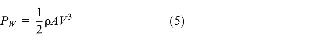
The potential wind power (P_W) is

P_{W} = \frac{1}{2} ρ A V^{3}

(5)

Hence, C_p is the ratio of the shaft power over the potential wind power.

The Reynolds number is an important factor that has great impact on the mechanical efficiency of a VAWT. This parameter can be calculated as follows

Re = \frac{ρ V_{1} d}{μ}

(6)

where d is the characteristic length of the turbine, which is the diameter of the wind turbine, and µ is the viscosity coefficient. V₁ is the wind speed in the flow field.

Tip speed ratio (TSR), defined below, is another important parameter, which is used in analyzing wind turbine performance

TSR = \frac{R ω}{V}

(7)

where R is the blade radius.

In order to achieve turbulence closures, when the physical model of the study is turbulent, we should add the corresponding control equations.

The law of mass conservation equation. It is also known as the continuous equation indicating that the net mass of the inflow control body in the unit time is equal to the mass of the control body itself under the same conditions and can be expressed as follows

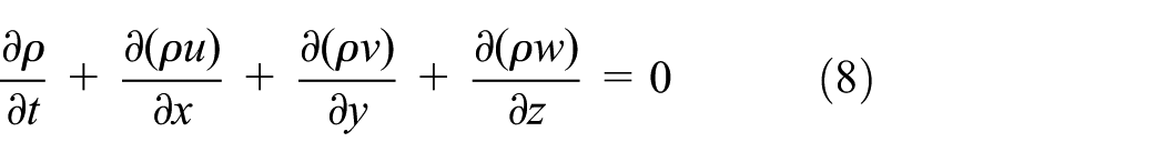
\frac{\partial ρ}{\partial t} + \frac{\partial (ρ u)}{\partial x} + \frac{\partial (ρ v)}{\partial y} + \frac{\partial (ρ w)}{\partial z} = 0

(8)

which can also be expressed as

\frac{\partial ρ}{\partial t} + \nabla \cdot (ρ \vec{V}) = 0

(9)

where V is the speed vector, and u, v, and w are the representations of V along the x, y, and z directions, respectively; and ∇ is the symbol of divergence. $ρ$ is the fluid density.

2.The law of momentum conservation equation. If there is no external force or the sum of external forces is 0, the overall momentum maintains the original value. The expression is given as follows

\begin{matrix} \frac{\partial (ρ u)}{\partial t} + \frac{\partial (ρ u^{2})}{\partial x} + \frac{\partial (ρ uv)}{\partial y} + \frac{\partial (ρ uw)}{\partial z} = - \frac{\partial p}{\partial x} \\ + \frac{\partial}{\partial x} (π λ \vec{\nabla} \cdot \vec{v} + 2 μ \frac{\partial u}{\partial x}) \\ + \frac{\partial}{\partial y} [μ (\frac{\partial v}{\partial x} + \frac{\partial u}{\partial y})] + \frac{\partial}{\partial z} [μ (\frac{\partial u}{\partial z} + \frac{\partial w}{\partial x})] + ρ f_{x} \end{matrix}

(10)

\begin{matrix} \frac{\partial (ρ v)}{\partial t} + \frac{\partial (ρ uv)}{\partial x} + \frac{\partial (ρ v^{2})}{\partial y} + \frac{\partial (ρ vw)}{\partial z} = - \frac{\partial p}{\partial y} \\ + \frac{\partial}{\partial x} [μ (\frac{\partial v}{\partial x} + \frac{\partial u}{\partial y})] \\ + \frac{\partial}{\partial y} (λ \vec{\nabla} \cdot \vec{v} + 2 μ \frac{\partial v}{\partial y}) + \frac{\partial}{\partial z} [μ (\frac{\partial w}{\partial y} + \frac{\partial v}{\partial z})] + ρ f_{y} \end{matrix}

(11)

\begin{matrix} \frac{\partial (ρ w)}{\partial t} + \frac{\partial (ρ uw)}{\partial x} + \frac{\partial (ρ vw)}{\partial y} + \frac{\partial (ρ w^{2})}{\partial z} = - \frac{\partial p}{\partial z} \\ + \frac{\partial}{\partial x} [μ (\frac{\partial u}{\partial z} + \frac{\partial w}{\partial x})] \\ + \frac{\partial}{\partial y} [μ (\frac{\partial w}{\partial y} + \frac{\partial v}{\partial z})] + \frac{\partial}{\partial z} (λ \vec{\nabla} \cdot \vec{v} + 2 μ \frac{\partial w}{\partial z}) + ρ f_{z} \end{matrix}

(12)

where $μ$ is the kinematic viscosity coefficient; f_x, f_y,and f_z are components of external forces, p is the pressure, λ is the second viscosity.

Modeling, meshing, and boundary condition setting

A VAWT system contains blades, a supporting pole, a generator, a drive shaft, and so on. To focus on the investigation of fluid–solid coupling and aerodynamic 3D model development of the blades, the permanent magnet generator and the drive shaft are integrated together. Figure 1 shows the Senegal-type turbine in the flow field which is simulated using ANSYS 3D CFX software. To simulate the real environment, the flow field of turbine model is divided into a stationary domain and a rotating domain. These domains are set to simulate the wind turbine working environment. The static domain is used to simulate a wide area of wind turbine farm environment; the rotating domain is for simulating the field with wind turbine blades. The height of wind turbine is set to 2 m; the inner diameter of blade is 1.7 m and the outer diameter is 1.9 m; the radius of the blade’s semicircular arc portion is 0.18 m; the plate length is 0.6 m; and the height of the pole is 3 m. In order to reduce the influence due to the flow field boundary upon the flow field, the static domain is set at a length of 7 m, a width of 4 m, and a height of 5 m (Figure 2).

Figure 1.

Senegal-type turbine in flow field.

Figure 2.

Wind turbine flow field boundary condition.

In the fluid field calculation, the mesh of the 3D model needs to be determined first. The fluid in the space is connected by points for calculation. In this work, the mesh generation is done automatically by the software (ANSYS), which is typical for most CFD studies. In this article, an automatic mesh generation method is adopted. The advantage of this method is that it has good performance in some irregular shapes. The mesh is relatively dense and has a tetrahedral shape. The total number of nodes ranges around 150 thousands, resulting in 780,000 mesh units. The first grid point is set in the logarithmic region; hence, the y⁺ value cannot be too small, which is set to 30. In this article, an adaptive method is used in this article. The essence of this method is to re-divide the grid according to the change of the stress gradient in the place where the stress gradient is large. As shown in Figure 3, the mesh becomes denser at the wind turbine in order to improve the calculation accuracy. Figure 3(a) represents the interface mesh and Figure 3(b) is the blade mesh, Figure 3(c) shows the mesh details of a single blade. In order to verify the accuracy of the simulation results, some verification of the model have been done in the previous studies.²¹ For example, the influence of the relative size of the static and rotating domains on the performance of the wind turbine, the influence of the position of the wind turbine in the fluid field and the mesh generation method on the performance of the wind turbine, and so on. This effect is mainly reflected in the coefficient of wind energy utilization and the coefficient of torque. The grid convergence verification and time step was also made in the previous studies, and the results show that when the grid number reaches over 480,000 and the steps are within 500, the calculation results are accurate. Due to the lack of actual data, the maximum wind energy utilization coefficient is sought by repeated change of model and repeated simulation studies. The accuracy is supported by these verifications.

Figure 3.

Meshing of the Senegal-type turbine.

One layer versus two layers

Figure 4 shows the basic structure of the one-layer wind turbine. Each layer of wind turbine consists of three blades, each of which is placed 120° apart. The proposed wind turbine is composed of two layers of wind blades. In order to simplify analysis, a wind turbine configuration of one layer with three evenly placed blades is investigated first. The Senegal-type turbine is simulated under a constant wind speed with different TSR (i.e. 0.141–0.78). The wind direction is shown in Figure 4, and the rotating direction of blades is clockwise from top view.

Figure 4.

3D model of the Senegal-type turbine.

Figure 5 shows the torque coefficient of a one-layer turbine in a whole rotating cycle. The TSR is set to 0.37, and the wind speed is 6.7 m/s. The initial position of the blade is shown in Figure 4. It can be seen from Figure 5 that the component forces of the three blades constitute the resultant force of the turbine, which has a rotation period of 120°.

Figure 5.

Torque coefficient of one layer of blades with wind speed 6.7 m/s.

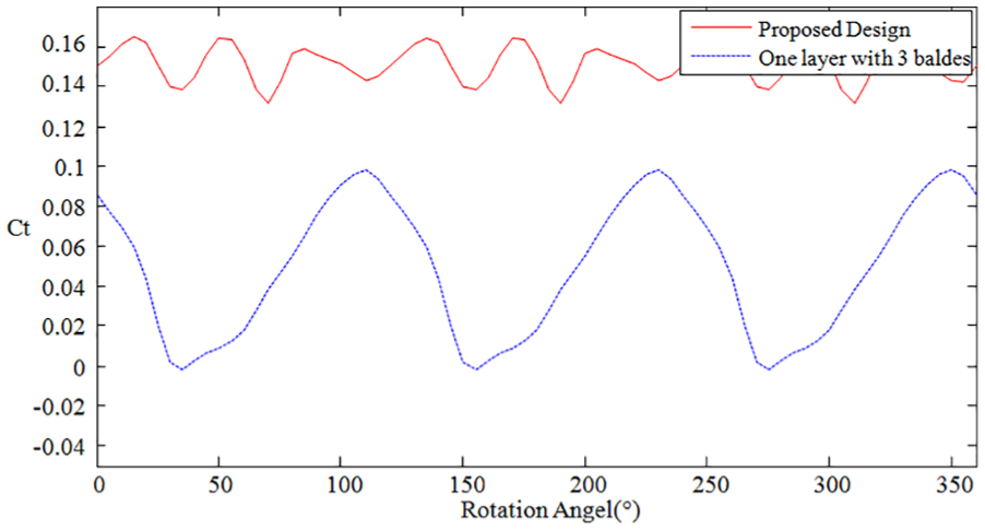
Figure 6 shows the torque coefficient curves of the one-layer design and the optimal model with two-layer design that will be discussed later. The torque coefficient presented here is the overall coefficient for all the blades. It is clearly shown in the figure that the curve of the one-layer design repeats every 120° since the three blades are evenly placed in space. It also can be seen from the figure that the one-layer design has very large, undesirable torque ripples/variations. Since the two-layer design with six blades can provide a much better torque output as shown in Figure 6, it (i.e. the proposed design) will be taken as the main structure for the wind turbine studied in this article. Detailed discussions on the two-layer design will be given in the following sections.

Figure 6.

Torque coefficient of two layers of blades with wind speed 6.7 m/s.

Boundary condition and simulation parameters

Based on the compressible continuous equation and Reynolds-averaged Navier–Stokes equation, the numerical calculation of wind turbine is carried out using ANSYS CFX. The angular velocity of the rotation domain is set up. The k-ε model is chosen as the model of turbulence. The wind turbine flow field consists two parts: the rotating domain and the static domain. The rotating domain is a flow field formed by the rotation of the wind turbine, which includes the wind blades, generator, and the rotating shaft. The static domain is the area where the air flows, including the supporting pole and the flowing air, which simulates the speed and direction of the incoming flow. The following inlet boundary condition is considered. Based on the real measurement data in the urban environment of Detroit, the following wind speeds are used in the simulation studies (4.9–18 m/s). In the inlet setting of boundary conditions, the wind is set to turbulent and the turbulent intensity is moderate. The outlet pressure is set to 0. The top and bottom boundary conditions are set to wall, and the two sides of the air domain are set to symmetry. The semi implicit method for pressure linked equations (SIMPLE) algorithm is chosen as the method of calculating the flow field, which takes into account the joint action of high-order solution and the upwind mode to achieve rapid convergence while ensuring the accuracy. The rotating field speed is set up with different values based on the different TSR (0.14–0.78 used in this study). Reynolds number (Re) also has an important effect on the accuracy of the results. In order to simulate the operation of the solid model more accurately, Re is calculated according to the actual environmental flow field. Other simulation parameters are summarized in Table 1.

Table 1.

Simulation parameters.

Reynolds number	Turbulence model	Iterations	No. of meshes	Residual target
6.0E+5	Standard k-ε model	150 steps	10 million	1.0E–4

Figure 7 shows the curves of C_p versus TSR under different wind speeds, where the Res are set at 490,000 (C_p1), 670,000 (C_p2), and 890,000 (C_p3), respectively. It can be found from Figure 7 that the wind energy utilization rate first increases and then decreases with the increase of TSR. The maximum value occurs when the TSR is between 0.5 and 0.6.

Figure 7.

Curves of power coefficient versus TSR under different Reynolds numbers.

Turbine structure design and selection

Different two-layer designs are investigated to choose an optimal design for improved torque and power performance. The turbine structure designs shown in Figures 8 and 9 show four blade structures namely, the closed plates, adding baffles inside, halving the length of plates (short plates in Figure 8(c)), and long plates, respectively. Figure 9 shows four different positioning styles of two layers of blades. The top layer of blades is positioned above the bottom layer by a certain degree, as shown in Figure 9. The angle difference between the two layers is 0° in the first scheme, while the angles are 20°, 40°, and 60° for the second, the third, and the fourth scheme, respectively. Based on the boundary conditions of the turbines, the cyclical data of the turbines’ torques are computed for the optimal designs.

Figure 8.

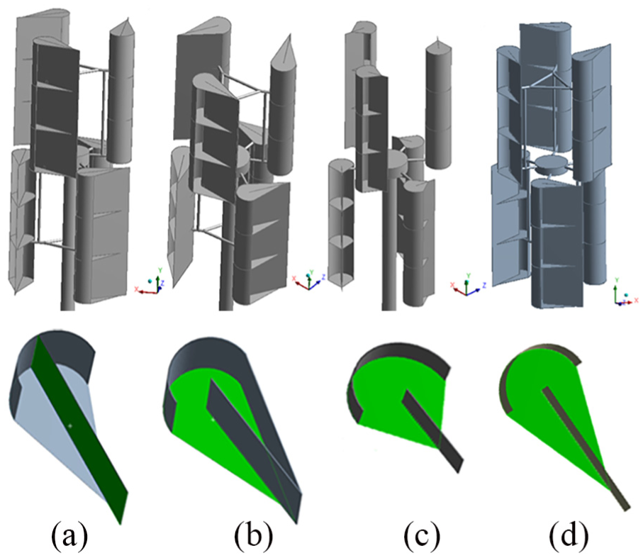
Four types of blade structures: (a) closed plates,(b) adding baffle plates, (c) short plates, and (d) long plates.

Figure 9.

Four top–bottom layer positioning schemes: (a) 0°, (b) 20°, (c) 40°, and (d) 60°.

Comparison of different blade designs

Figures 10 –13 show the two-dimensional (2D) force distribution on the two layers of turbines at a certain position (rotation angle) for the four types of blade structures shown in Figure 8. The top sub-figure in each figure shows the force distribution of the three blades in the top layer; the bottom one shows the force distribution of the three blades in the bottom layer. In these studies, the rotation angle is set at 70° because the largest torque coefficient (C_t) appears at this situation in one cycle, as shown in Figure 14. Figure 10 shows the force distribution of the closed plate blade structure in Figure 8(a). The right side of the top layer blades has a greater pressure, and the wind energy cannot be converted efficiently for driving. The whole pressure is concentrated on blades and against the steady turning of the turbine.

Figure 10.

2D force distribution of the closed-plates design.

Figure 11.

2D force distribution of the adding baffles design.

Figure 12.

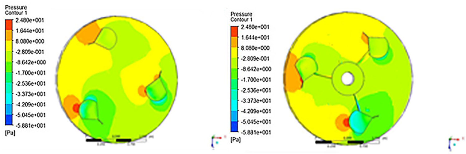
2D force distribution of the short-plates design.

Figure 13.

2D force distribution of the long-plates design.

Figure 14.

The torque coefficient curves in one full cycle for the four blade structures.

Figure 11 shows the force distribution for the adding baffles design in Figure 8(b). Compared with Figure 10, due to the blocking effects on the air flowing through the adding baffle plates, the force on the lower part of the top-left blade is significantly less than that of the design in Figure 10. For the same reason, the pressure exerted on the windward side of the blade is larger. This design of turbine has a greater utilization of the wind power near the blades, but the disadvantage lies in that it is easy to form a vortex due to the non-conducive feature for the wind flow, which makes it against capturing wind energy in a dynamic process.

Figure 12 shows the result of the scheme of halving the length of the plates. Compared with Figure 10, the pressure on the right side of the top layer blades is similar, but the pressure is also larger on the bottom layer of turbine due to the lack of plate barrier effects by the blades. Generally, the torque is smaller than the scheme shown in Figure 10.

Figure 13 shows the force distribution for the scheme by using long plate blades (Figure 8(d)). The top blades have bigger resistance in producing torque, but the bottom ones are in the better position. This structure can produce a fairly good torque as a whole.

It can be observed from Figures 10 –13 that the proposed blade structure of long plates in Figure 8(d) can produce the highest torque. To better illustrate this, the torque coefficients of the four blade schemes during one cycle are shown in Figure 14. It can be seen that the proposed scheme of long plates has the best performance in terms of torque coefficient, while the scheme of adding baffles scheme shows the smallest torque value.

Comparisons of different top–bottom positioning schemes

Figure 15 shows the torque coefficient curves of the four positioning schemes between the top and bottom layers of blades. The angle α between the top and the bottom layers is changed from 0° (Scheme 1), 20° (Scheme 2), 40° (Scheme 3), and 60° (Scheme 4, the proposed one), respectively. When the offset angle α is greater than 60°, since there are three blades evenly placed in each layer, the equivalent offset angle is (120°–α). Thus, the maximum positioning offset angle between the top and bottom layers is 60°. The curves in Figure 14 were obtained under the condition when TSR is 0.57 and wind speed is 6.7 m/s.

Figure 15.

Comparison of the four placement schemes of top and bottom blade layers.

It can be seen in Figure 15 that the torque coefficient curve of Scheme 1 has a period of 120° in terms of angle while the curve of Scheme 4 has a period of 60°. Scheme 1 has the highest peak value of C_t, but the blades are subject to the strongest compressive force and the biggest force ripples, which accelerate the process of material fatigue. There are even some negative values of C_t in some positions for Scheme 1. To achieve a more stable and smoother output torque, Scheme 4 is chosen for implementing the VAWT.

Simulation results and experimental studies

3D simulation studies have also been carried out to investigate the performance of the proposed VAWT. The overall output power curve at different wind speeds is obtained via the simulation studies. The simulation result is compared with the actual measured data (Figure 26) of a 2-kW VAWT that was built and installed on the roof of the Engineering Technology Building in Wayne State University (WSU) based on the design.

Flow field analysis

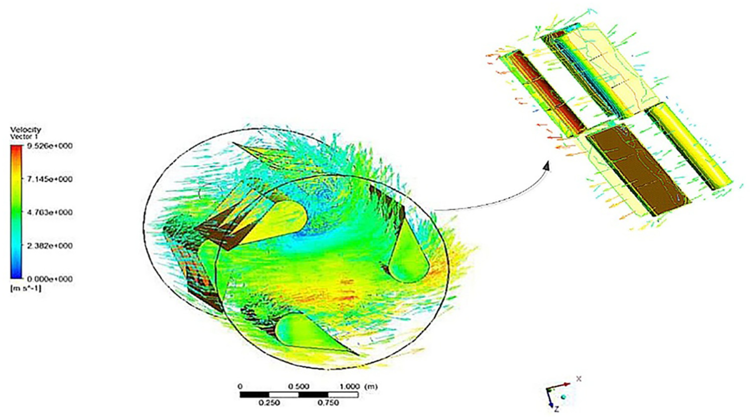
In this simulation, the wind velocity vector is set along the axis of positive direction. The simulation is done under the situation when wind speed is 6.7 m/s and TSR is 0.57.

According to the wind velocity vector distribution in Figure 16, the wind energy loss is reduced due to the top and bottom block plates of blades. Within the middle section of the rotating field between the two layers, the wind speed slows down owing to the turbulence. The turbulence is in clockwise direction and weakens the pressure of wind to the blades and also reduces the turbine’s efficiency. Meanwhile, from the upper section of blades in the figure, the air flow passes between the plate and semi-cup, accelerating the flowing of the flow field. This design improves the utilization of wind energy by reducing the impact of turbulence.

Figure 16.

Wind velocity vector distribution of the turbine model.

For a more intuitive understanding of wind speed on the turbine, in the CFD post-processing, the velocity contours are shown in Figures 17 and 18.

Figure 17.

Wind velocity contour of the top layer of blades.

Figure 18.

Wind velocity contour of the bottom layer of blades.

When the wind blows, the semi-disk side of the blade suffers a greater resistance. The blades are exerted with the resistance difference of the windward side to implement rotation motion.^21–24 Disproportion of airstream will produce the thrust force to move around the blades. In Figure 16, the thrust force of blades is smaller owing to the slower wind speed around the turbine, while the middle section of blades loses part of wind energy on account of high wind speed. The wind fields of the bottom layer blades, marked as 1, 2, and 3 in Figure 18, are more complicated than those of Figure 17. Because of the obstruction effect caused by the supporting pole, the wind speed around blade 3 is smaller. The 2D and 3D velocity contours can reflect the wind field around the wind turbine. The 2D velocity contour selects a section of the wind field, which is convenient to study the wake and the wind velocity of the wind turbine at a certain height. The 3D velocity contour can better reflect the details of the wind inside the wind turbine and the overall pressure of the wind turbine. Comparing the 3D and 2D results, it can be seen that the wind speed inside the wind wheel is obviously disordered and lower than the top and bottom, and the wind speed gradually recovered after two diameters of the turbine on the downstream side. Figures 19 and 20 show the sectional views of the wind velocity flow distributions of the top and bottom layers, respectively.

Figure 19.

Velocity flow distribution of the top blades.

Figure 20.

Velocity flow distribution of the bottom blades.

It can be seen from Figure 18 that the velocity is reduced in the vicinity of the blades. Meanwhile, the streamline in the left side passes through the blade and goes down, ultimately comes as turbulence before the blade. The turbulence makes the left blade suffer high-speed shock impact and reduce the drag effect on the right blade to improve C_p. In Figure 20, the direction of rotation is anti-clockwise. The turbulence appears at the upper left blade and the front of the lower blade because of the obstructive plate, which leads to the wind velocity beneath the plate greater than on top of the plate. According to Bernoulli principle, the pressure beneath the plate is greater than at the top, producing greater power.

Analysis of torque coefficient results

The torque under a constant wind speed of 6.7 m/s is calculated for different TSR values, as given in Table 2. The results of the torque are the average values in one cycle.

Table 2.

Simulation results at the wind speed of 6.7 m/s.

Parameter name of the wind turbine	The value of the parameter
TSR	0.14	0.28	0.37	0.47	0.57	0.67	0.78
ω (rad/s)	0.77	1.54	2.03	2.56	3.08	3.66	4.23
Torque (N·m)	111.8	101.2	80.4	70.1	60.7	47.2	22.6

TSR: tip speed ratio.

Under a constant wind speed of 6.7 m/s, the torque is calculated when the turbine rotates every 10°. The torque coefficient curve over 360° is shown in Figure 21. The torque coefficient curve has a period of 120°, and the peak is reached at around 70°. Figure 22 is the velocity distribution when the turbine rotates 70°, at which the torque coefficient reaches its peak value.

Figure 21.

C_t curve of turbine rotation cycle at TSR = 0.57.

Figure 22.

Velocity vector of the turbine at the rotation position of 70°.

Wind turbine implementation and experimental studies

Based on the proposed structure of VAWT given in Figures 8(d) and 9(d), a 2-kW VAWT has been built on the roof of the Engineering Technology Building in WSU, as shown in Figure 23. The characteristic length (d) of the turbine is 2.494 m. The system has been in full operation since June 2011. The system has a Davis Vantage Pro 2 weather station and 16-channel data acquisition (DAQ) system to measure and store weather data (wind velocity, temperature, etc.) and various circuit quantities such as current, voltage, and power from the VAWT. A website (http://hres.eng.wayne.edu/) has been developed to share the real-time data (every minute) of the system with researchers worldwide. The data can be useful for carrying out research on harvesting wind energy in urban environments. The DAQ system for this wind turbine mainly consists a personal computer (PC) with a Texas Instrument (Dallas, Texas) (TI) PCI-MIO-16xe-10 DAQ card,²⁵ a TI SCB-68 interface box, and voltage and current sensors. The sampling resolution of the PCI card is 16 bit. LEM HAL 100-S hall-effect current transducers are used to measure the currents. The accuracy of the current transducer is ±1%.²⁶ Customized resistive voltage dividers are used to measure the voltages with an accuracy of ±1%. We have installed the voltage and current sensors to measure the output voltage and current of each phase of the permanent magnet synchronous generator (PMSG) of the wind turbine. The measured current and voltage values are used to calculate the wind output power. The overall accuracy of the power measurement (three-phase) is then about 2.5%.

Figure 23.

Prototype of the proposed Senegal VAWT.

The actual wind turbine system installed at WSU is not equipped with TSR control. The wind turbine has a PMSG. Hence, its output voltage is proportional to the rotating speed. Figure 24 shows the system diagram, where the output of the wind turbine generator is rectified into DC to charge a 48 V/48 kWh battery bank. Since the battery terminal voltage is relatively constant, the output voltage of the wind turbine increases with the turbine rotating speed when the wind speed increases as the current increases and the voltage drop between the battery and the generator output increases. However, the turbine output voltage as well as the rotating speed does not change much since the equivalent resistance between the wind turbine and the battery is not large. Figure 25 shows the power electronic converters for the wind turbine. And the power output of the wind turbine is simulated. The simulation is completed using ANSYS Workbench and MATLAB. First, the model of the Senegal wind turbine was built using ANSYS Workbench, and the torque results at different wind speeds were calculated. The results were imported to the PMSG model in MATLAB, and the output voltage and power were obtained by torque input.

Figure 24.

The schematic diagram of the wind turbine system at WSU.

Figure 25.

The power electronic converters for the wind turbine system.

Table 3 shows the data of the practical output power and the simulation results. The actual measured wind power at different wind speeds is given in Figure 26. The simulation results are compared with the measured data to test the accuracy of output power by prediction, as shown in Figure 26 when TSR is set as 0.57. As a result, the power density of the proposed VAWT can be as high as 20 W/m²,²⁷ which is about 7–10 times higher than that of a typical HAWT.²⁸ From the figure, it can be seen that the simulated output power curve is in accordance with the measured data. In general, the simulated wind power is slightly higher than the measured data. The deviation is in a reasonable range which can be caused by certain power losses, such as the power losses of the bearing and power converter, and such losses are not included in the simulation study. Moreover, there are differences between the simulated flow field and the actual flow field, and the simulated flow field is ideal. In fact, due to the obstacles of the surrounding buildings and other complex natural conditions, there can be discrepancies between the simulation results and the actual results.

Table 3.

The data of the practical output power and the simulation results.

Parameter name of the wind turbine	Power data at different wind speeds
Wind speed (m/s)	4	4.8	5.8	6.7	7.6	8.95	10.3	11.2	12.1	13.4	14.7	15.7	16.5	17.9
Practical output power (W)	101	92	93	112	160	139	152	161	162	251	400	638	624	910
Simulated output power (W)	65	69	92	123	124	171	188	196	208	294	492	573	750	970

Figure 26.

The output power of the turbine.

Wake stream influence on the turbine

VWATs can be installed on the roof of buildings in an urban environment. The impact upon the turbine performance caused by nearby buildings and other turbines need to be studied. Figure 27 shows the simulated velocity flow around the proposed VAWT (see the top figure). The wind speed is 10 m/s with a TSR of 0.5 for the simulation study. According to the right figure, the area of upwind is the primary section which has a great influence on the wind speed behind the blades.

Figure 27.

Velocity flow diagram in the wind field.

Figure 28 shows the impact caused by nearby objects on the implemented turbine, which is about 5 m above the roof. The top figure shows that the impact caused by the roof and the objects on the roof is negligible; the bottom figure shows the effects of obstacle objects such as a chiller tower near the turbine. It can be seen from the top figure, the roof has less influence on the turbine; and according to the bottom figure, when there is an obstacle in front of the turbine, the wind turbine flow field can be influenced, thereby reducing the power of the turbine.

Figure 28.

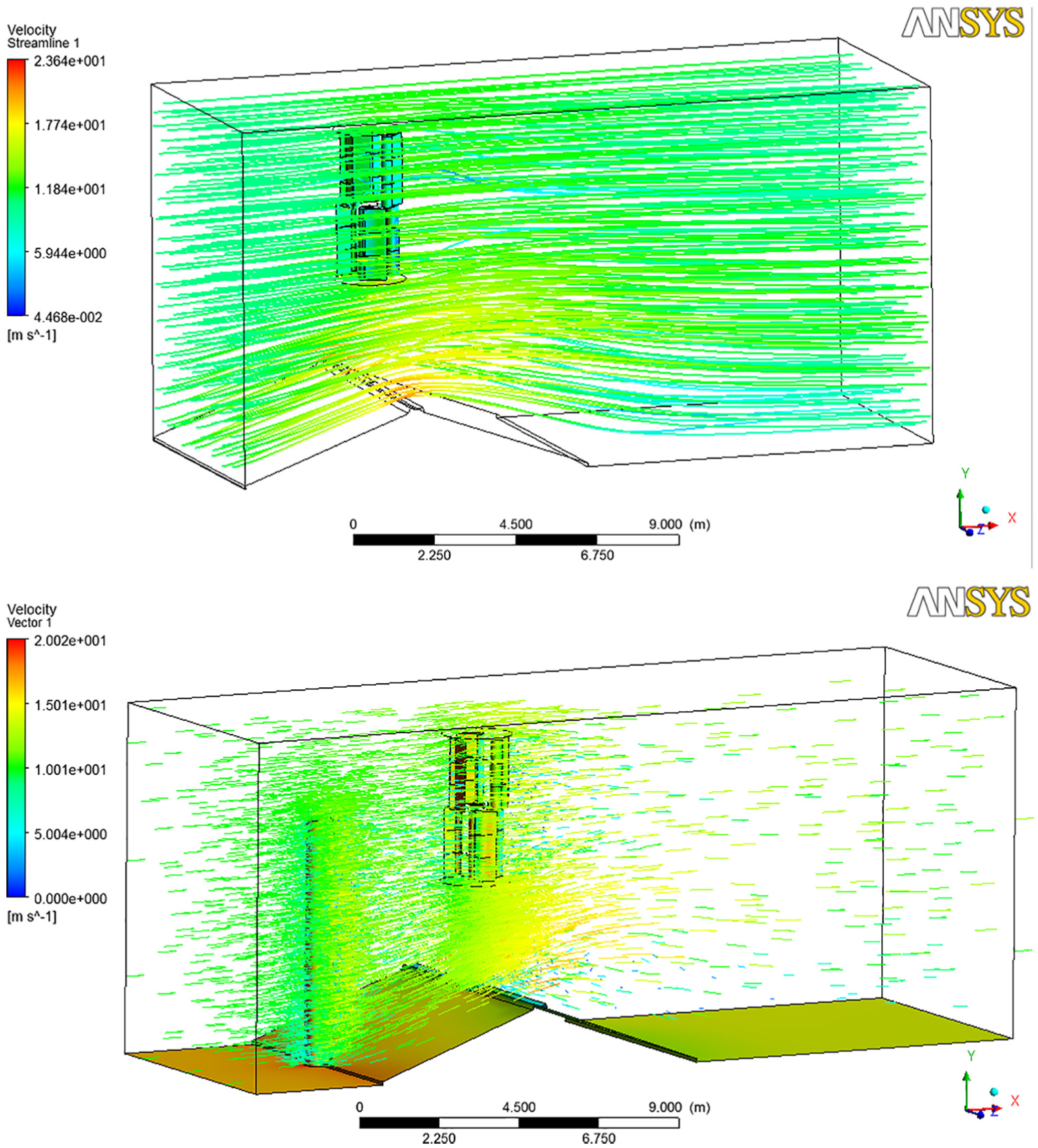
Obstacle impact of buildings.

Through the calculation and experiments, in the workbench post-processing 3D graphics, the result shows in Table 4 that when the wind speed is around 10 m/s while the TSR is 0.57, the length of the turbine’s wake effect is roughly around 6 m, which is about two-diameter distance between the centers of two VAWTs in any direction. This distance is much shorter than the typical placement distance between two HAWTs, which is six to eight times of the turbine diameter. This interesting feature of VAWT enables the possibility of developing a hybrid wind farm consisting of HAWTs and VAWTs for better wind energy utilization and higher power density.

Table 4.

Torque at the wind speed of 10 m/s with and without the obstacle.

	Without the obstacle	Obstacle half-diameter distance away from turbine	Obstacle one-diameter distance away from turbine	Obstacle two-diameter distance away from turbine
Torque (N m)	125	61	95	119
C_p	0.134	0.024	0.078	0.13

Conclusion

A CFD 3D model of a drag-type VAWT has been developed in the article. The developed model has been used to investigate the impact of design parameters on the turbine performance. Four different blade structures and four positioning schemes of the two layers of blades have been studied to choose an optimal design. A 2 kW prototype system has been implemented based on the optimal design. The effectiveness of the 3D models and simulation results has been verified by the measured data from the actual VAWT system that has been in operation since 2011. The wake effects acting on the VAWT caused by nearby objects have been also investigated. The simulation results show that the proposed VAWT has a small wake loss if the turbine placement distance is over two turbine diameters. The actual operation experiences also show that the proposed system has the characteristics of low cut-in speed, omni-directional wind energy capture, and robustness to adjacent objects (such as buildings and other wind turbines), which make it suitable for small-scale wind energy systems in populated areas including urban environments.

Footnotes

Acknowledgements

The authors acknowledge the help from Kelso Energy Ltd for implementing the vertical wind turbine system on the roof of the Engineering Building at Wayne State University.

Handling Editor: Jiin-Yuh Jang

Declaration of conflicting interests

The author(s) declared no potential conflicts of interest with respect to the research, authorship, and/or publication of this article.

Funding

The author(s) disclosed receipt of the following financial support for the research, authorship, and/or publication of this article: This work is supported by the National Natural Science Foundation of China (grant nos.: 51577048, 51877070, and 51637001), the Natural Science Foundation of Hebei Province of China (grant no.: E2018208155), the Overseas Students Science and Technology Activities Funding Project of Hebei Province (grant no.: C2015003044), the Hebei Industrial Technology Research Institute of Additive Manufacturing (Hebei University of Science and Technology) open projects funding, the National Engineering Laboratory of Energy-saving Motor & Control Technique, Anhui University (grant no.: KFKT201804), and the Key Project of Science and Technology Research in Hebei Provincial Colleges and Universities (grant no.: ZD2018228). The work of C.W. was supported in part by the National Science Foundation of USA under grant no. ECCS-1508910.

ORCID iD

Zheng Li

References

Feng

Chen

et al . A simulation and experimental research on aerodynamic characteristics of combined type vertical axis wind turbine. Acta Energiae Solaris Sinica 2014; 35: 855–860.

Max

Conaill

Alex

Comparison of power electronics lifetime between vertical- and horizontal-axis wind turbines. IET Renew Power Generat 2016; 10: 679–686.

Richard

Larry

Toward the coevolution of novel vertical-axis wind turbines. IEEE Trans Evol Comput 2015; 19: 284–292.

Lei

Liu

Yang

. Performance comparison for Savonius type wind turbines by numerical analysis approaches. In: Proceedings of the 2015 international conference on advanced mechatronic systems, Beijing, China, 22–24 August 2015, pp.402–406. New York: IEEE.

John

OD.

Potential order-of-magnitude enhancement of wind farm power density via counter-rotating vertical-axis wind turbine arrays. J Renew Sustain Energy 2011; 3: 043104.

Shaheen

Abdallah

Development of efficient vertical axis wind turbine clustered farms. Renew Sustain Energy Rev 2016; 63: 237–244.

Maeda

Kamada

et al . Investigation of power performance and wake on a straight-bladed vertical axis wind turbine with field experiments. Energy 2017; 141: 1113–1123.

Wang

Nehrir

Analytical approaches for optimal placement of distributed generation sources in power systems. IEEE Trans Power Syst 2004; 19: 2068–2076.

Stotsky

Egard

Carlson

. Control of wind turbines: a tutorial on proactive perspectives. In: Proceedings of the American control conference (ACC), Washington, DC, 17–19 June 2013, pp.3429–3436. New York: IEEE.

10.

Zhao

Wang

Zhao

et al . A review of active management for distribution networks: current status and future development trends. Elect Power Compon Syst 2014; 42: 280–293.

11.

Shafii

Obermaier

Linn

et al . Visualization and analysis of vortex-turbine intersections in wind farms. IEEE Trans Visualizat Comput Graph 2013; 19: 1579–1591.

12.

Schluter

. Design and analysis of small-scale vertical axis wind turbine. In: Proceedings of the IET conference on renewable power generation (RPG), Edinburgh, 6–8 September 2011, pp.1–10. New York: IEEE.

13.

Placide

Francois

Alain

. Aerodynamic and mechanical system modeling of a vertical axis wind turbine (VAWT). In: Proceedings of the IEEE conference on electrical and control engineering, Yichang, China, 16–18 September 2011, pp.5189–5192. New York: IEEE.

14.

Kou

Shi

Yuan

et al . Modeling analysis and experimental research on a combined-type vertical axis wind turbine. In: Proceedings of the 2011 international conference on electronics, communications and control (ICECC), Ningbo, China, 9–11 September 2011, pp.1537–1541. New York: IEEE.

15.

Chang

Hsu

Miao

et al . Numerical studies of the flowfield over a hybrid VAWT with different torque. In: Proceedings of the international conference on consumer electronics, communications and networks (CECNet), Xianning, China2011, pp.5077–5081. New York: IEEE.

16.

Arpino

Cortellessa

Dell’Isola

CFD simulations of power coefficients for an innovative Darrieus style vertical axis wind turbine with auxiliary straight blades. J Phys 2017; 923: 012036.

17.

Kludzinska

Tesch

Doerffer

. An experimental and numerical study on the performance of an innovative vertical-axis wind turbine. In: Proceedings of the VII European congress on computational methods in applied sciences and engineering, Crete, 5–10 June 2016, pp.1–8. Barcelona: ECCOMAS.

18.

Kumar

Micha Premkumar

Seralathan

Numerical investigation of modified Bach type vertical axis wind turbine. Appl Mech Mater 2016; 852: 551–557.

19.

Wen

Liu

JT.

Study on working mechanism of directional efficient vertical axis wind turbine. J Inner Mongolia Agri Univ 2016; 6: 78–84.

20.

Yang

Pan

Zhu

HQ.

An overview and recent research progresses of vertical axis wind turbine. China Mech Eng 2013; 24: 703–709.

21.

Gao

Sun

TT.

Numerical simulation and analysis of vertical axis wind turbine characteristics in distributed energy system. Trans China Electrotech Soc 2017; 32: 155–163.

22.

Veers

Ashwill

Sutherland

HJ.

Trends in the design, manufacture and evaluation of wind turbine rotor. Wind Energy 2003; 6: 245–259.

23.

Duquette

Visser

KD.

Numerical implications of solidity and blade number on rotor performance of horizontal-axis wind turbines. J Solar Energy Eng 2003; 125: 425–432.

24.

Xie

Wang

TG.

Modification of calculating unsteady aerodynamic characteristics of wind turbine rotor. Eng Mech 2008; 25: 54–59.

25.

PCI-MIO-16XE-10. (PCI-6030), http://www.ni.com/documentation/en/multifunction-io-device/latest/pci-mio-16xe-10/overview/

26.

Current Transducer HAL, https://www.darrahelectric.com/media/documents/HAL_Series.pdf

27.

Gao

PF.

Research on small vertical axis wind turbine modeling and generation characteristics. Shijiazhuang, China: Hebei University of Science and Technology, 2016.

28.

Wang

Yan

Aerodynamic analysis of impellers of horizontal axis variable pitch wind turbine. J Northeast Univ 2010; 31: 1178–1181.

Analysis and implementation of a drag-type vertical-axis wind turbine for small distributed wind energy systems

Abstract

Keywords

Introduction

Modeling of drag-type VAWT

Characteristic parameters

Modeling, meshing, and boundary condition setting

One layer versus two layers

Boundary condition and simulation parameters

Turbine structure design and selection

Comparison of different blade designs

Comparisons of different top–bottom positioning schemes

Simulation results and experimental studies

Flow field analysis

Analysis of torque coefficient results

Wind turbine implementation and experimental studies

Wake stream influence on the turbine

Conclusion

Footnotes

Acknowledgements

Declaration of conflicting interests

Funding

ORCID iD

References