Sage Journals: Discover world-class research

Abstract

Driving force analysis is performed on the no-spin differential and full-time all-wheel-drive vehicle; this thesis takes an automatic loading mixing vehicle as an example to introduce the compositions and working principle of the driving system. Based on the tire-ground mechanics, the model of the dynamics and the kinematics is established under the walking straight and steering conditions. According to the theoretical model, the influence of the vehicle’s gravity center on the moving system is analyzed. Co-simulation based on LMS Imagine Lab AMESim and LMS Virtual Lab Motion is performed to build the hydraulic driving system and the multi-body dynamics system models. Based on the tire-ground load environment simulation model built by 1D + 3D, various positions of the gravity center of the model are set to compare with the theoretical analysis. Various weight blocks are also added to change the location of the gravity center in the practical experiment. The conclusions that different gravity center positions lead to the change of the driving torque distribution are proved by the simulation results and experimental data.

Keywords

No-spin differential and full-time all-wheel-drive vehicle 1D + 3D co-simulation gravity center driving torque distribution LMS Imagine Lab AMESim

Introduction

According to a lot of material out there, almost all travel driving forces originate from the contact between the vehicle and ground.¹ In this context, it is meaningful and feasible to study the interaction between the tire and ground during the design process of wheeled vehicles. The automatic loading mixing vehicle is taken as the research object in this article, which belongs to the no-spin differential and full-time all-wheel-drive vehicle (ND&AWD). The mechanical theory model should be established, not just for the study of the interaction between the tire and ground but for the further investigation of the dynamics and kinematics. Based on the tire mechanical characteristics and the relationship between the center of gravity distribution and the driving force, simulation and experiments are carried out.

Fundamentals of driving system

The automatic loading mixing vehicle adopts hydromechanical composite transmission system. On one hand, the hydraumatic part is a closed system, including variable capacity pump, reversing motor, relief valve, overflow valve of oil filling, pilot control oil circuit, washing oil circuit, and the fuel tank. On the other hand, the mechanical part is composed of transfer case, drive axle, and tires. As shown in Figure 1, the traveling of the vehicle is realized by diesel engine with variable-speed governor and variable pump of speed-sensitive control.

Figure 1.

Hydraulic schematic of automatic loading mixing vehicle’s driving system.

While the car is in motion, the power of the engine is transferred to the variable pump in the main oil circuit. The motor can output torque and speed because of the pressure difference between them (e.g. if the high pressure oil comes out of port B, the port A is the low pressure port), which realizes the transmission of energy. The pressure difference on both sides of A and B increases when the traveling resistance becomes larger on account of the sudden heavy load. When the target goes up to a certain extent, the pressure signal will be sent from pressure sensor of travel motor to PLUS1 controller of variable pump, and then the PLUS1 controller will give the corresponding signal to shift solenoid valve of motor, which will change the displacement of motor from small to large. As a result, the status of the vehicle is low speed and high torque, which can help overcome the heavy load. However, if the heavy load still cannot be conquered, system pressure will continue to rise, and the relief valve of the main circuit will open once the pressure difference on both sides of A and B is greater than the relief pressure. At this point, the pressure of the system is released and the pilot needs to shift gears. When the vehicle needs to be towed on account of moving system failure, the main shaft of motor can be freely rotated by opening two bypasses of the main variable pump to connect the high and low pressure side.

Tire-ground mechanics principle

Ground features of tire

The automatic loading mixing vehicle in this article belongs to wheeled vehicle, and the ultimate executing mechanism is the pneumatic tire. The moving performance of vehicle is derived from the connection between inflatable tires and the ground, and the structural parameters of the tire and the different loading conditions will have a direct impact on the sliding deformation of tire.¹ Thus, the effective rolling radius of vehicle in motion is affected. At this point, the distribution of tire driving force of the vehicle is changed. The main cause of rolling resistance is the deflection of tire, which will directly affect its mechanical properties on the ground. Tire slip deformation is that when the tire is driven by torque, the tread is compressed before entering the contact area of the ground. At this point, the rolling radius of the tire is smaller when the torque is driven; in other words, the transverse moving distance becomes small. This phenomenon is called the slip deformation of the tire.

Radius $r_{0}$ is that the tire is free and has no load on it, which is called the free radius of the tire. When the vehicle is motionless, the tire is only subjected to the radial load during normal inflation. The vertical distance from the tire center to the ground is the static radius $r_{s}$ .²

r_{s} = r_{0} - Δ z

(1)

where $Δ z$ indicates deflection, m.

The vertical distance of its geometric center to the ground is referred to as the effective rolling radius of the tire $r_{m}$ when the tire is in pure rolling motion without sliding under external force. The research shows that when the rotation speed of the tire is low, the load on the tire has a large influence on the no-slip rolling radius of the tire, and the mixer vehicle is a low speed vehicle. Therefore, the effective rolling radius of the tire is approximately equivalent to the static radius of the tire $r_{m}$ .³

r_{m} = r_{s} - Δ z

(2)

where $r_{0}$ indicates rolling radius of the tire, m; $r_{m}$ denotes effective rolling radius of the tire, m; and $r_{s}$ represents static radius of the tire, m.

The experiments conducted by Jilin University and Changchun Automobile Research Institute show that the shape of the tire near the ground is mostly between the ellipse and the rectangle, but for engineering mechanical tires, when the load is especially large, its grounding shape is closer to the rectangle. For the convenience of numerical analysis, the grounding shape is simplified as a rectangle, as shown in Figure 2. Integrating the experimental results of different tires with the deformation characteristics of the tire,⁴ Automobile Ground Mechanics Institute of Jilin University proposed the following empirical formula to calculate the length of the tire grounding rectangle X and width Y, as shown in equations (3) and (4)

X = 4 R {(\frac{Δ z}{2 R})}^{κ}

(3)

Y = T (1 - e^{- λ Δ z})

(4)

where $κ, λ$ indicate empirical coefficient, dimensionless; T denotes tire crown width, m; e represents base of natural logs, dimensionless; and R indicates tire radius, m.

Figure 2.

Schematic diagram of tire deformation.

The above studies prove that the contact area of tire touching the ground is shown below

S = XY

(5)

where S indicates the area of the tire touching the ground, $m^{2}$ ; and H denotes the vertical load on the tire, kN.

The stress on the ground is shown as follows

σ = \frac{H}{S}

(6)

where $σ$ represents grounding pressure, kPa.

Fujimoto studied the radial deflection of the tire with the vertical load, and the radial deflection of the tire under the determined vertical load is shown as follows⁵

Δ z = z_{0} + ϕ H

(7)

where $ϕ$ indicates relation coefficient of the tire structure, MPa

ϕ = \frac{c_{2}}{{(p_{t} + p_{i})}^{c_{1}}}

(8)

where $c_{1}$ , $c_{2}$ , and $z_{0}$ are the constants associated with the tire structure, dimensionless; $p_{t}$ represents pressure caused by stiffness of the tire, MPa; and $p_{i}$ indicates pneumatic pressure of the tire, MPa.

Carrying equation (8) into equation (7), the following equation is figured out

Δ z = z_{0} + \frac{c_{2}}{{(p_{t} + p_{i})}^{c_{1}}} H

(9)

Inserting equation (9) into equations (3) and (4), the following equations are obtained

X = 4 R {(\frac{z_{0} + \frac{c_{2}}{{(p_{t} + p_{i})}^{c_{1}}} H}{2 R})}^{κ}

(10)

Y = T (1 - e^{- λ (z_{0} + \frac{c_{2}}{{(p_{t} + p_{i})}^{c_{1}}} H)})

(11)

Driving force and the slip rate of the wheel

When the tire is driven, the friction force is formed because of the relative movement between the tire and the ground, which causes the corresponding shear deformation. In order to predict the relationship between the driving force and the slip rate of the wheel, it is necessary to specify the distribution of the shear displacement along the wheel ground and the relationship between shear force and shear displacement which is calculated by Bekker formula (12)^6–9

\begin{matrix} ζ = (C + σ \tan φ) (1 - e^{(- h / k)}) \\ = ζ_{\max} (1 - e^{(- h / k)}) \end{matrix}

(12)

where $ζ$ represents the tire shearing stress, MPa; C denotes the cohesion of the material, $N$ ; $φ$ indicates the shear strength angle of the material, °; h denotes the tire shear displacement, m; and k represents the shear modulus, MPa.

As the direction of the shear stress between the wheel and the ground is consistent with the direction of the vehicle movement.¹⁰ According to the torque balance, it can be seen that the driving resistance of the vehicle under linear driving conditions is the shear resistance of the integral on the whole contact surface, which can work out the driving resistance on each tire. Based on the balance of torque, the tire driving force is equal to its resistance from the ground, so the driving force can be calculated as follows¹¹

\begin{matrix} F_{q} = \int ζ dS = \int_{- X / 2}^{X / 2} \int_{- Y / 2}^{Y / 2} ζ dXdY \\ = \int_{- X / 2}^{X / 2} \int_{- Y / 2}^{Y / 2} (ζ_{\max} (1 - e^{(- h / k)})) dXdY \end{matrix}

(13)

where $F_{q}$ represents driving force of the vehicle, N.

The distribution of vehicle weight

The load on the tire of mixer vehicle mainly comes from the vehicle’s gravity. If the center of gravity of the mixer vehicle is not in the geometric center of the space hexahedron formed by the four tires, the load on the four tires must be different from the weight of the vehicle. It can be seen from the “Ground features of tire” section that the contact area between the tire and the ground is closely related to the vertical load on the tire. In this article, the center of gravity of the mixer vehicle is tilted to the rear axle in longitudinal direction, while the weight distribution on the horizontal direction is basically symmetric. Therefore, the model can be simplified as the horizontal center of gravity in the middle; the center of gravity in the longitudinal direction $(Δ G)$ is located at the intersection of the diagonal of the quadrangle (the quadrangle is formed by the grounding center of four tires when all tires are set) and adjacent to the rear axle. The simplified model and its tire forces are shown in Figure 3.

Figure 3.

Wheel-ground shear action diagram.

Due to the symmetry of gravity distribution in the transverse direction, the radial loads on the two tires connected to the same axle are equal with each other. The torque balance equation is applied to the front axle center of the vehicle in the longitudinal direction (i.e. Figure 4); the vertical loading of the front and rear tires can be obtained

G_{f} + G_{r} = G

(14)

G_{r} L = G (\frac{L}{2} + Δ G)

(15)

where $G$ indicates vehicle center of gravity, $N$ ; $G_{f}$ denotes front axle vertical load, $N$ ; $G_{r}$ represents rear axle vertical load, $N$ ; L indicates wheelbase between the front and rear axles, m; and $Δ G$ denotes distance from the gravity center to geometry center, m.

Figure 4.

Schematic diagram of vehicle gravity center.

The distribution of the vehicle load on each tire is shown as follows

G_{t_{1}} = G_{t_{2}} = \frac{G_{f}}{2} = \frac{\frac{L}{2} - Δ G}{2 L} Δ G

(16)

G_{t_{3}} = G_{t_{4}} = \frac{G_{r}}{2} = \frac{\frac{L}{2} + Δ G}{2 L} Δ G

(17)

where $G_{t_{1}}, G_{t_{2}}, G_{t_{3}}, G_{t_{4}}$ represent the vertical load of the left front tire, right front tire, left and right rear tire, $N$ .

Analysis of straight line walking conditions

The linear moving condition is one of the typical and common conditions for automatic loading mixing vehicle. Under this linear moving condition, the vehicle’s chassis system is powered by the engine, which transmits the power to the walking variable pumps, and then to the walking motors, gearboxes, bridges, and eventually to the tire. As a result, there is no axial differential device in the process of transmission to the front and rear axles, as shown in Figure 5

V_{j 1} = v

(18)

where $V_{j 1}$ indicates speed of right front wheel center, m/s; and v denotes vehicle speed, m/s.

Figure 5.

Schematic diagram of straight line walking conditions.

As shown in Figure 6, the speed of the center of the contact area between tire and ground during sliding can be expressed as follows

V_{s_{1}} = r_{m_{1}} ω - v

(19)

where $V_{s_{1}}$ indicates the speed of the center of the contact area, m/s.

Figure 6.

Speed of tire slip diagram.

The relationship between the shear displacement and the slip speed of the tire is a complex nonlinear; however, in the case of steady work, the displacement in the x direction increases with the rise of sliding speed, which is approximately a linear relationship. In this case, the linear substitution curve is adopted to present the internal action relationship. The shear displacement formula at any point in the ground area of the tire can be expressed as follows

h_{1} = β v_{s_{1}}

(20)

where $β$ indicates the relation coefficient of tangential deformation and slip velocity, dimensionless.

Similarly, the displacement formula of a point in the ground area of the other three tires can be obtained

V_{s_{i}} = r_{m_{i}} ω - v

(21)

h_{i} = β v_{s_{i}}

(22)

where i indicates two, three, and four tires.

The study shows that the tire stiffness $p_{c}$ is related to the load of the tire

p_{t} = ψ H

(23)

where $ψ$ indicates conversion factor, $1 / m^{2}$ .

It can be seen from Figure 6 that the driving force of the vehicle in a straight line is determined by the displacement of the wheel, and the wheel shear displacement mainly depends on the speed of the slip. The difference between the sliding speed of tire 1 and tire 3 is available

\begin{matrix} V_{s_{1}} - V_{s_{3}} = (r_{m_{1}} ω - v) - (r_{m_{3}} ω - v) \\ = ω (r_{m_{1}} - r_{m_{3}}) \\ = ω {\begin{matrix} [r_{s} - (z_{0} + \frac{c_{2} G_{t 1}}{{(ψ G_{t 1} + p_{i})}^{c_{1}}})] \\ - [r_{s} - (z_{0} + \frac{c_{2} G_{t 3}}{{(ψ G_{t 3} + p_{i})}^{c_{1}}})] \end{matrix}} \\ = ω (\frac{c_{2} G_{t 3}}{{(ψ G_{t 3} + p_{i})}^{c_{1}}} - \frac{c_{2} G_{t 1}}{{(ψ G_{t 1} + p_{i})}^{c_{1}}}) \end{matrix}

(24)

As shown in equation (24), with the same physical parameters of two tires, the difference between the slip speeds of the two tires is closely related to the vertical load of the tires. The larger differences between the vertical load of each tire, the greater discrepancies between the sliding speed of each tire, and the driving force will be different. Equation (24) shows that once the size of the ground area is ignored, the condition (if $G_{1} > G_{3}$ , then $v_{s_{1}} > v_{s_{3}}$ ) is valid; in other words, the driving force of tire 1 is greater than tire 3. It indicates that the position of the gravity center of the vehicle influences the driving force distribution of the front and rear wheels, which will be further proved in the following simulations and experiments.

Simulation

Build of simulation model

AMESim was used as the modeling and simulation platform of engineering systems in many fields.^12–14 The simulation model of the walking driving system of the automatic loading mixing vehicle is established based on the AMESim in this article, as shown in Figure 7. The main variable pump and variable motor are modeled in the walking driving system.

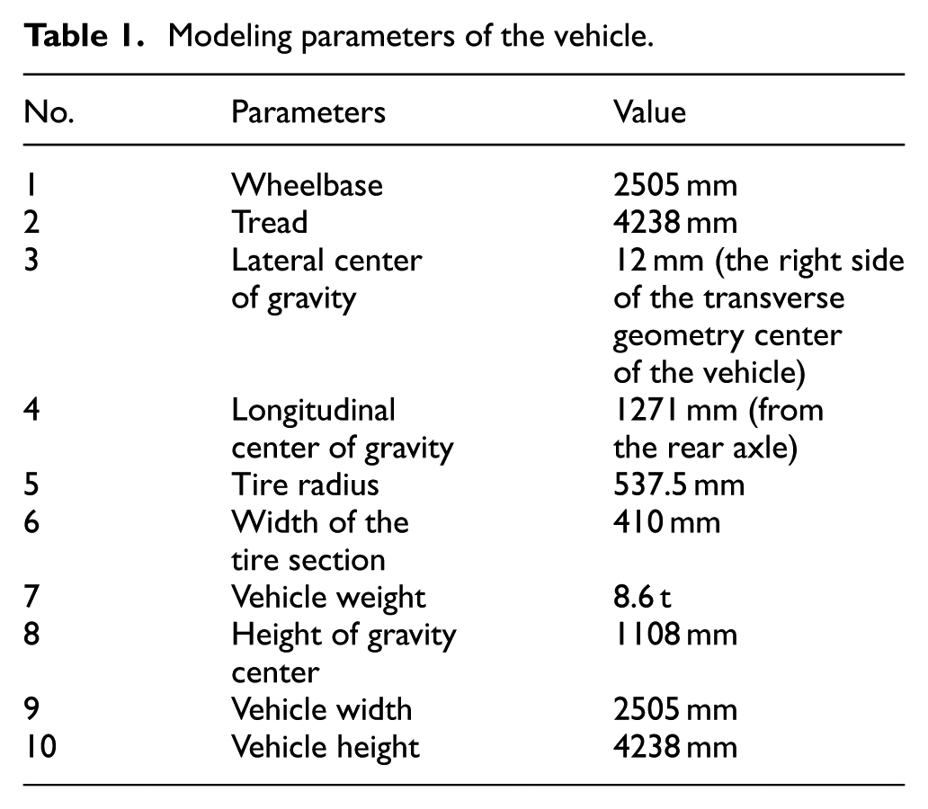
In Motion, multi-body dynamic modeling of the mixer vehicle is carried out. First, the three-dimensional model is established in ProE, in order to ensure the vehicle center of gravity position; heterogeneous components can be equivalent to lumped mass block. Second, the four tires are assembled and added constraints in Motion with the vehicle.¹⁵ Finally, the hard ground condition is set in Motion. The main modeling parameters of the vehicle model are shown in Table 1, and the motion constraint relationship is shown in Table 2. The motion model diagram is shown in Figure 8.

Figure 7.

AMESim model of travel driving system.

Table 1.

Modeling parameters of the vehicle.

No.	Parameters	Value
1	Wheelbase	2505 mm
2	Tread	4238 mm
3	Lateral center of gravity	12 mm (the right side of the transverse geometry center of the vehicle)
4	Longitudinal center of gravity	1271 mm (from the rear axle)
5	Tire radius	537.5 mm
6	Width of the tire section	410 mm
7	Vehicle weight	8.6 t
8	Height of gravitycenter	1108 mm
9	Vehicle width	2505 mm
10	Vehicle height	4238 mm

Table 2.

Constraint relationship.

No.	Mechanism 1	Mechanism 2	Motion pair	Quantity	Remark
1	Tire	Steering knuckle	Cylindricalvice	4	Everytire

Figure 8.

Motion model.

This model mainly focuses on the impact of tire load on driving force, which involves the modeling of tire and its parameter setting. The tire models included in Motion are as follows:^16–18 simple tire, complex tire, Systems Technologies Inc (STI) tire, magic formula tire, and so on. According to the requirements of this study, the simple tire model is selected, and the hard ground road conditions are set in Motion, and then tire-ground forces are added to the tire and ground. The final parameter values are shown in Figure 9.

Figure 9.

Setting of final parameter values in Motion: (a) Set of road in Motion, (b) the model with weight block in Motion, (c) set of tire structure parameters, and (d) set of tire control parameters.

Defining the ratio of the distance from the gravity center position to the center line of the front axle and rear axle as Longitudinal Gravity Center Distance Ratio (LoR), at the same time, the ratio of the center of gravity to the distance of the center line of the left tire and right tire is defined as Lateral Gravity Center Distance Ratio (LaR). The position of gravity center of the vehicle studied in this article is 5.4:4.6 (LoR) and 4.9:5.1 (LaR).

Simulation based on different conditions

Straight moving condition

The simulation is based on the flat cement road. The complete working cycle of the straight moving condition is described as follows.

First, start the engine and set the gearbox to second gear (the gear ratio is 26.85), and set the variable motor as 80 mL/r. Second, input the walking signal to start the mixer vehicle. Third, input the stop signal to the engine after a period, and then the mixer vehicle stops working. Finally, the vehicle simulation is finished.

1. Longitudinal gravity center impact on the moving system

In the study of longitudinal position simulation, five models of different LoR are established, and five ratios are 3:7, 4:6, 5:5, 6:4, and 7:3, respectively.

As shown in Figure 10 and Table 3, the data of the vehicle moving system change with different ratios.

Figure 10.

Torque curve for different LoR: (a) LoR = 3:7, (b) LoR = 4:6, (c) LoR = 5:5, (d) LoR = 6:4, and (e) LoR = 7:3.

Table 3.

Simulation data of different LoR.

LoR	Front axletorque (Nm)	Rear axle torque (Nm)	The total torque of the vehicle (Nm)	Torque ratio of front and rear axles
3:7	388	1684	2072	1.9:8.1
4:6	628	1447	2075	3:7
5:5	1015	1038	2053	4.9:5.1
6:4	1431	651	2082	6.9:3.1
7:3	1680	374	2054	8.2:1.8

In Figure 10, curves 1, 2, and 3 represent front axle, rear axle, and torque of the whole vehicle.

It can be seen from Figure 10 that the torque of the front axle increases gradually from 388 to 1680 Nm as the center of gravity is shifted longitudinally, while the rear axle torque decreases from 1684 to 374 Nm. During this process, the driving torque of the vehicle is stable. It shows that the position of center of gravity has great influence on the torque distribution of the front axle and rear axle, but it has little influence on the total driving torque of the whole vehicle.

Through the analysis of the ratio of the front axle and rear axle torque, its ratio also goes from small to large with the backshift of gravity center. The values of the first column and the last column in Table 3 indicate that the trend is consistent, but they do not establish linear relationship.

2. Lateral gravity center impact on the moving system

In the lateral position simulation, five models of different LaR are established, and five ratios are 3:7, 4:6, 5:5, 6:4, and 7:3, respectively. The initial and operational process of the mixer vehicle is exactly the same as that of the longitudinal center of gravity.

As shown in Figure 11 and Table 4, the stable mean and change trend of the front axle torque, rear axle torque, and the driving torque of the whole vehicle are also consistent with different ratios.

Figure 11.

Curve of different LaR.

Table 4.

Hectometer lateral deviation of various LaR.

LaR	3:7	4:6	5:5	6:4	7:3
Hectometerlateraldeviation	4.8 left	1:1 left	0.1 left	0.8 right	4.6 right

In Figure 11, curve 1 and curve 2 are the drive torque of the front axle and rear axle at different LaR, respectively, and curve 3 is the total vehicle torque at different LaR.

From the above table, it indicates that different LaR corresponds to different levels of lateral deviation in the 100-m walking process. When the LaR is 5:5, the vehicle lateral migration does not occur, but it will vary with the change of lateral center. In other words, the lateral deviation is related to the horizontal center of gravity position, and the larger the shift of the horizontal center of gravity, the larger the lateral deviation.

The above analyses show that the horizontal center of gravity position has no effect on the front axle, rear axle, and the vehicle driving force, but it will cause the vehicle side bias in the process of walking. As a result, the position of lateral center of gravity has a significant influence on driving safety.

Steering condition

For further analysis of the relationship between the driving force and gravity center, the steering condition is adopted. Then, the whole dynamic moving cycle is formed by straight moving and steering conditions.

The steering condition simulations are divided into two groups: front wheel steering mode and four-wheel steering mode, which are all based on the flat cement road. The complete working cycle of steering condition is described as follows.

First, start the engine and set the gearbox to second gear, set the variable motor as 80 mL/r. Second, input the walking signal to start the mixer vehicle, and then turn the steering wheel to rotate the tires to a certain angle; after that, drive the mixer vehicle to walk in circles. Third, input the stop signal to the engine after a period and turn the steering wheel to return the tires; then the mixer vehicle stops working. Finally, the vehicle simulation is finished.

According to the structure of the vehicle, it is obvious that the vehicle gravity center changes once the tires rotate. Considering the difficulty in measuring of gravity center and the diversity of deflection angle in the actual experiment, the turning radius is taken as the index of reference. The greater the angle of deflection of the tire, the smaller the steering radius and the greater change in the position of the gravity center.

1. Front wheel steering condition

As shown in Figure 12 and Table 5, the simulation data of front wheel steering mode are reached.

Figure 12.

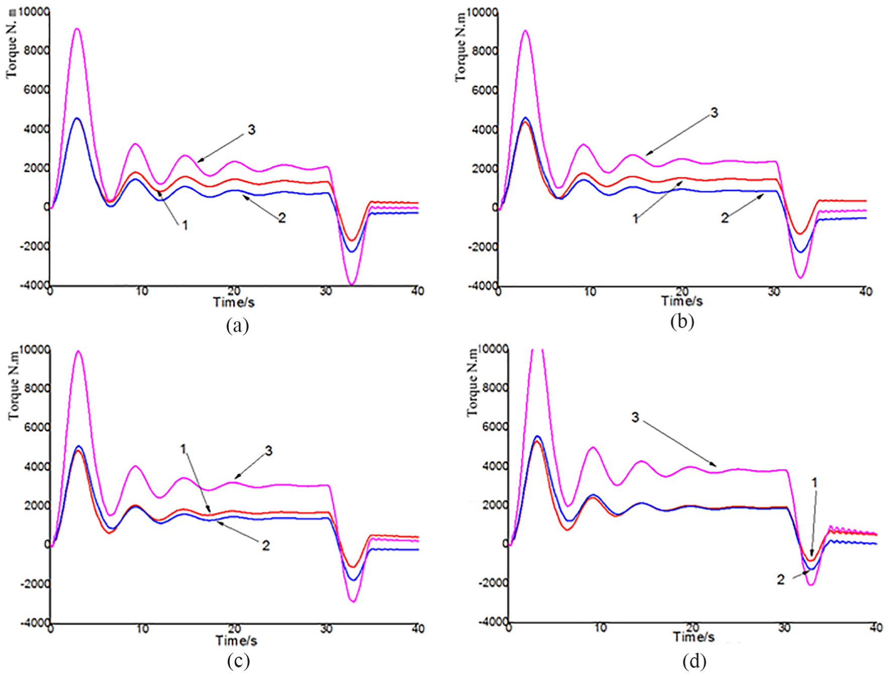
Torque curve for front wheel turning radius: (a) turning radius, 0 m; (b) turning radius, 8.8 m; (c) turning radius, 6.6 m; and (d) turning radius, 4.7 m.

Table 5.

Distribution of driving torque with various turning radii (front wheel steering).

Turning radius/m	0	8.8	6.6	4.7
Front axle/Nm	1379	860	170	−702
Rear axle/Nm	805	1883	3569	5663
The total torque of the vehicle	2184	2743	3769	4961
Ratio of front and rear axles	6.3:3.7	3.2:6.8	0.05:9.95	−0.12:100

It can be seen in Figure 12 that different turning radii lead to different distribution of driving force between front and rear axles. Furthermore, with the decrease of steering radius, the driving force values of front axle even become negative, which means that the front axle plays a role in the load at that time.

2. Four-wheel steering condition

As shown in Figure 14 and Table 6, the simulation data of the four-wheel steering mode are captured.

Table 6.

Distribution of driving torque with various turning radius (four-wheel steering).

Turning radius/m	0	8.8	6.6	4.7
Front axle/Nm	1379	1516	1698	1937
Rear axle/Nm	805	922	1373	1851
The total torqueof the vehicle	2184	2738	3081	3788
Ratio of frontand rear axles	6.3:3.7	6.2:3.8	5.5:4.5	5.1:4.9

Analyzing Figure 12 with Figure 13, it can be found that the difference in the distribution of driving forces is smaller under the condition of the same change rate of turning radius in four-wheel steering condition. The driving force values are always positive. Such differences appear because the four-wheel steering mode has less influence on the gravity center position than the two-wheel steering mode.

Figure 13.

Torque curve for four-wheel turning radius: (a) turning radius, 0 m; (b) turning radius, 8.8 m; (c) turning radius, 6.6 m; and (d) turning radius, 4.7 m.

Experiment and analysis

As shown in Figure 14, this article takes the EWH3.5-A as a prototype vehicle designed by HIGH-TECH Shandong Heavy Industries Co., Ltd. During the experiment, strain gauge and DH5905 (wireless torque test module) are attached to the transmission shaft first, and then the DH5905 collects and transmits the torque through wireless router; finally, the signal is displayed on the computer. Due to the limit of experimental conditions, only the front axle torque is used for comparison and analysis.

Figure 14.

Experiment scene: (a) experiment equipments for torque test, (b) demonstration vehicle, and (c) position of DH5905 on transmission shaft.

Experiment of straight moving

The straight moving experiment is conducted, as shown in Figure 15. Figure 16 shows the experimental results.

Figure 15.

Mixer vehicle in straight moving condition.

Figure 16.

Front axle torque comparison of straight moving: (a) vehicle without weight block; (b) vehicle with the weight block in the rear, and (c) vehicle with the weight block in the front.

The loads on the tires are changed through the position shift of the 600 kg weight block on the automatic loading mixing vehicle. When the weight block is in the rear of the vehicle, the output torque of the front axle is 1350 Nm. However, as the weight in the bucket, the front axle torque is reduced by about 50 Nm. On one hand, it can be clearly seen from Figure 17 that when the engine is just starting, the simulation curves have a big torque mutation; this is because the engine in simulation is at a low speed and high torque state to overcome the travel resistance torque. For actual experiment, the vehicle is in the state of engine idling to stabilize the vehicle state at the initial phase. On the other hand, the overall trend of the experimental curves is the same as the simulation curves, and some of the differences are due to the errors caused by some irresistible factors (such as signal acquisition error, road random disturbance).

Figure 17.

Mixer vehicle in steering condition.

The test shows that the load ratio of the front axle and rear axle has a certain effect on the output torque of the front axle and rear axle of the vehicle. When the overall weight of the mixer vehicle does not change, the forward motion of the center of gravity will reduce the driving torque of the front axle, which is basically consistent with the previous theoretical analysis and simulation.

Experiment of steering condition

The steering condition experiments are conducted, as shown in Figure 17. Figure 18 shows the experimental results.

Figure 18.

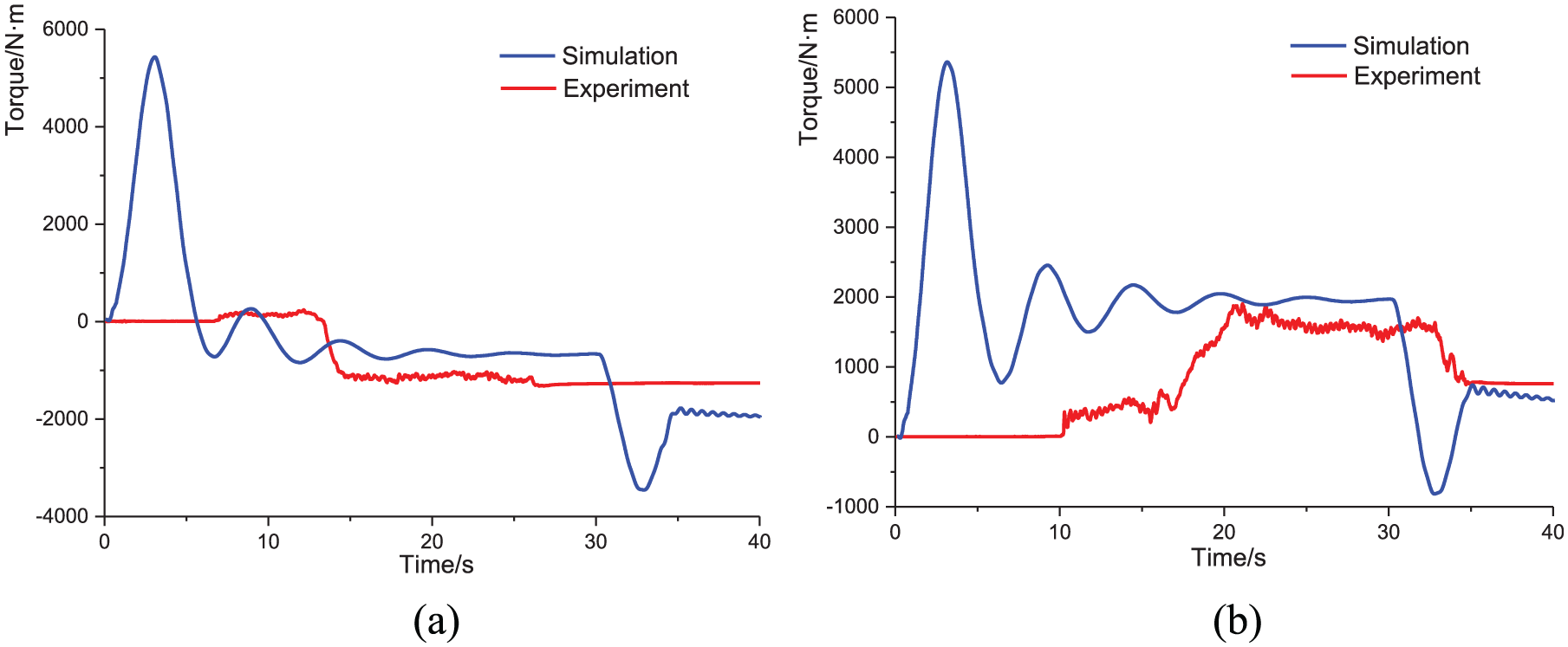
Experimental curves of front axle for steering condition: (a) front axle torque comparison of front wheel steering and (b) front axle torque comparison of four-wheel steering.

As shown in Figure 18(a), the trends of the experiment and simulation curves are consistent roughly, which shows that the simulation is effective and suitable. Based on Figure 18(b), it can be seen that both of them are positive, which means that the front axle is always producing the driving force. In addition, both of the two curves in Figure 18(a) and (b) are different in the initial period (0–10 s), which is caused by the differences in start-up phases between experiment and simulation. During the process of actual experiment, from 0 to 10 s, the vehicle is in the state of engine idling to stabilize the vehicle state, thus forming a more obvious contrast with the steering action. For the simulations, the vehicle model starts directly at 0 s, which leads to a big shock. From 10 to 40 s, the differences between simulation and experiment in Figure 18 are caused by ground disturbances, sensor error, vehicle handling error, and so on.

As described in the “Steering condition” section, the four-wheel steering mode has a smaller influence on the center of gravity than the front wheel steering mode. Thus, in the process of front wheel steering, the front axle acts even as load rather than drive source when the gravity center moves back to a certain extent. In conclusion, the experiments are basically consistent with the previous theoretical analysis and simulation.

Conclusion

This article analyzes the impact of gravity center’s position on ND&AWD (such as the automatic loading mixing vehicle) in detail, and a Motion-AMESim simulation model is established according to the actual structure parameters.

Combining the theory principle, simulation models, and experiment analyses, it indicates that the driving forces vary with the change of the gravity center of the vehicle when the total weight of the vehicle is constant. And the drive axle far away from the center of gravity drives more torque.

This article fills the gap of the theory validation, that is, the center of gravity has an impact on the distribution of ND&AWD’s driving force . These conclusions reveal that it is important to take the gravity center position into consideration during the vehicle design process.

Footnotes

Acknowledgements

We are also grateful to the anonymous referees and the editor-in-chief for their suggestions to improve this paper.

Handling Editor: Michal Kuciej

Declaration of conflicting interests

The author(s) declared no potential conflicts of interest with respect to the research, authorship, and/or publication of this article.

Funding

The author(s) disclosed receipt of the following financial support for the research, authorship, and/or publication of this article: This paper is supported by the university–industry collaboration project under Grant No. 3R114D222414.

ORCID iD

Chen Zhou

References

Wong

. Some problems in the mechanics of soil-wheel interaction. In: Proceedings of the 3rd international conference of the International Society for Terrain Vehicle Systems, vol. 1, Essen, Germany, 9–12 July 1969.

Han

Zhou

Sun

The research of the factors impacting on the tire rolling radius. J Agric Mech Res 2017; 1: 163–166.

The research of the dynamic radius and slip of the driving wheel. Tract Farm Transp 2003; 2: 17–20.

Zhuang

Tires for cars. Beijing, China: Beijing Institute of Technology Press, 2001.

Zhuang

Automobile tire science. Beijing, China: Beijing Institute of Technology Press, 1996.

Bekker

MG.

Introduction to terrain-vehicle systems. Ann Arbor, MI: The University of Michigan Press, 1969.

Wong

. The theory of ground vehicles (Library of Congress cataloging-in-publication data). 3rd ed. Wiley-Interscience, 2009, p.560.

Huang

Principle of ground vehicles. Beijing, China: China Machine Press, 1985.

Krick

Radial and shear stress distribution beneath rigid wheels and pneumatic tyres on yielding soils with regard to tyre deformation. J Terramechanics 1969; 6: 73–98.

10.

Zhang

Yang

Geometrical condition analyses of four-wheel vehicle skid-steering. Tract Farm Transp 2007; 6: 12–14.

11.

Pacejka

Sharp

RS.

Shear force development by pneumatic tyres in steady state conditions: a review of modelling aspects. Vehicle Syst Dyn 1991; 20: 121–175.

12.

Wei

Yin

Modeling and simulation of aircraft nose landing gear emergency lowering using co-simulation method. Advances in Design Technology Vols, 1 and 2 2012; 215-216: 1213-1218

13.

Liang

Ning

Shi

Simulation research of fin stabilizer hydraulic system based on AMESim and ADAMS co-simulation. Tract Farm Transp 2009; 8: 200–202.

14.

Liu

Modeling and simulation for the hydraulic system based AMESim. Xi’an, China: Northwestern Polytechnical University, 2006.

15.

Zhang

On dynamic modeling of mechanical pair clearance. Xi’an, China: Xidian University, 2006.

16.

Zhao

The simulation and experimental study of the hydraulic steering system for loader. Changchun, China: Jilin University, 2012.

17.

Wan

Introduction to LMS virtual.lab motion. Xi’an, China: Northwestern Polytechnical University Press, 2010.

18.

Dugoff

Segel

Fancher

PS.

An analysis of tire traction properties and their influence on vehicle dynamic performance (SAE Transactions). New York: Society of Automotive Engineers, 2013.

Distribution of driving force beneath wheeled vehicle with varying center of gravity

Abstract

Keywords

Introduction

Fundamentals of driving system

Tire-ground mechanics principle

Ground features of tire

Driving force and the slip rate of the wheel

The distribution of vehicle weight

Analysis of straight line walking conditions

Simulation

Build of simulation model

Simulation based on different conditions

Straight moving condition

Steering condition

Experiment and analysis

Experiment of straight moving

Experiment of steering condition

Conclusion

Footnotes

Acknowledgements

Declaration of conflicting interests

Funding

ORCID iD

References