
Abstract
Robot position accuracy plays a very important role in advanced industrial applications. This article proposes a new method for enhancing robot position accuracy. In order to increase robot accuracy, the proposed method models and identifies determinable error sources, for instance, geometric errors and joint deflection errors. Because non-geometric error sources such as link compliance, gear backlash, and others are difficult to model correctly and completely, an artificial neural network is used for compensating for the robot position errors, which are caused by these non-geometric error sources. The proposed method is used for experimental calibration of an industrial Hyundai HH800 robot designed for carrying heavy loads. The robot position accuracy after calibration demonstrates the effectiveness and correctness of the method.
Keywords
Introduction
In the off-line programming (OLP), the joint angles are desired to achieve a given Cartesian position of the arm’s tip by using a kinematic model of the robot arm. However, a nominal geometrically model according to a product specification sheet does not include the errors arising in manufacturing or assembly. In addition, it also does not include non-geometric errors, such as gear transmission errors, gear backlashes, and arm compliance, which are difficult to geometrically consider in a kinematic model. Therefore, some methods of calibrating precisely kinematic and non-kinematic parameters are required to improve the accuracy of robot manipulators.
Previously published studies have focused on modeling robot error sources for purposes of calibration.1–12 These errors are classified into two types: geometric errors and non-geometric errors. Geometric errors include link twist angle errors, link length errors, link offset, and joint angle offsets. Non-geometric errors include gear backlash, joint deflection, and link compliance. Some researchers have focused on kinematic model of robots but took into account only geometric errors.3–7 Other researchers8,9 developed robot kinematic models that included both link geometric and non-geometric errors (only joint deflection). 10 However, there are other non-geometric error sources that significantly affect the robot accuracy; therefore, we cannot leave out any non-geometric error parameters. Some research has suggested that robot joint deflection and link compliance affect position accuracy.11,12 The deformation of robot joints and links is due to robot link weights and carried payloads. Previously, Duelen and Schroer 11 applied a theory of flexible beams to investigate the effects of robot link compliance. These effects were demonstrated by changing six differential elements (three for translation changes and three for rotation changes). Hudgens et al. 12 utilized a methodology for identifying general robot deflection characteristics under applied torques and forces. These methods resorted to special tools and sensors for finding compliance error elements. Both works11,12 should include other non-geometric errors for more accurate robot calibration.
Recently, the extended Kalman filter (EKF) algorithm, 13 genetic algorithm, 14 maximum likelihood estimation,15,16 particle filter (PF) algorithm, 17 and Fourier polynomials 18 are also applied for identifying non-linear kinematic parameters. Some researchers have been developing the hybrid calibration algorithms; Jiang et al. 17 suggested a combination algorithm, including the EKF and PF. This research was based on the EKF algorithm providing a priori value, and the PF algorithm was used to calibrate the robot kinematic parameters. Although the method has advantages of working for high dimensional systems, it still has some drawbacks. It does not include the non-geometric error sources such as link compliance, gear backlash, and other. Alici and Shirinzadeh 18 applied Fourier polynomial for compensating the non-geometric error. Although, these methods were successfully used in robot calibration, they do not supply knowledge of error sources in robot structure, have slow convergence, and the calibration space is limited. Artificial neural networks (ANNs) have also been widely used for approximating non-linear relationships in systems or industrial robots because of their advantageous properties such as learning ability, adaptation, and flexibility. Some researchers have applied the ANN to compensate for robot position errors.19–23 Jang et al. 19 used a radial basis function network (RBFN) to form a functional relation to describe the robot joint offset errors in terms of their joint positions. The works19,21 have utilized an ANN in order to describe the functional relationship of end-effector positions and corresponding position errors. However, the position errors essentially depend on robot configurations. It has been proven in previous works24,25 that a robot can approach a given Cartesian coordinate with multiple configurations and each configuration will produce a different position error. The work 22 has applied a multiple layer ANN to approximate the relationship between robot joint positions and associated joint offset errors. The application of ANN for robot error compensation still has some shortcomings because a user cannot know the robot error sources. However, some errors can be modeled easily and correctly, for example, the robot link geometric errors and the robot joint compliance are easily modeled.
The model-based calibration method, mentioned above, has many advantages such as less computing time, fast convergence, and accurate knowledge of error sources. Some error sources (especially non-geometric errors) cannot, however, be determined and modeled correctly. Therefore, the robot position error, which is caused by these error sources, should be compensated for by using an ANN. The combination of both model-based calibration and ANN compensation methods can be an effective solution for enhancing robot position accuracy.
In this article, we present a technique for the calibration of industrial robots by combining the advantages of the two above methods. The first one is a model-based calibration method and the second is position error compensation using an ANN. First, we model and identify robot kinematic error parameters, including geometric errors and joint compliance errors. Second, the robot residual position errors, which are caused by other non-geometric errors such as link deflection and gear backlash, are compensated for by using an ANN. By comparing with the work, 19 the proposed method can also include the robot joint compliance errors in the robot model. The ANN, which was built with the proposed method, also described a more appropriate relationship between the robot joint readings and its end-effector positions instead of the unsuitable one used in the work. 19 Experimental calibration for the Hyundai HH800 robot was carried out to demonstrate the effectiveness and correctness of the proposed method.
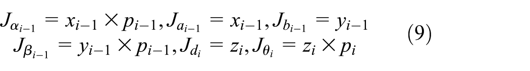
The remainder of the article is organized as follows. The “Kinematic model of the HH800 robot” section develops a robot kinematic model for use in calibration. The “Formulation for parameter identification” section derives formulas for the identification of robot kinematic parameters, including geometric parameters and joint compliance. The “ANN and its application for robot position error compensation” section constructs an ANN and shows how to compensate for the robot position errors. The “Experiment and results” section describes experimental calibration and results. Finally, some conclusions are presented in the “Conclusion” section.
Kinematic model of the HH800 robot
This section describes kinematic model for the Hyundai HH800 robot (Figure 1). The “Kinematic model of HH800 robot” section describes building the robot kinematic model and the “Robot joint compliance model” section describes modeling the robot joint compliance.

A sketch of the HH800 robot and its link frames.
Kinematic model of HH800 robot
The 6 degrees of freedom (dof) HH800 robot, which is described in Figure 1, consists of a main open kinematic chain (6 dof) and a closed-loop mechanism (2 dof). The open chain is connected by the revolute joints 1, 2, 3p, 4, 5, and 6. The closed-loop PQRS is connected by the revolute joints 2, 3, Q, R, and S (both joints’ axes 2 and 3 are coincident at point P). The frames are fixed at the open chain’s links based on the Denavit–Hartenberg (D-H) convention. 26 The nominal D-H parameters of the open chain and the closed loop are shown in Table 1.
D-H parameters of HH800 robot (units: length (m), angle (°), “–”: unavailable).

D-H: Denavit–Hartenberg.
A transformation matrix of two consecutive link frames {i – 1} and {i} is computed by
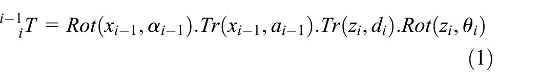
where robot link parameters include the twist angle
A homogeneous transformation from the robot base frame to the end-effector frame, which describes the pose of the end-effector with respect to the base frame, is computed as follows

where

The matrix

and the matrix
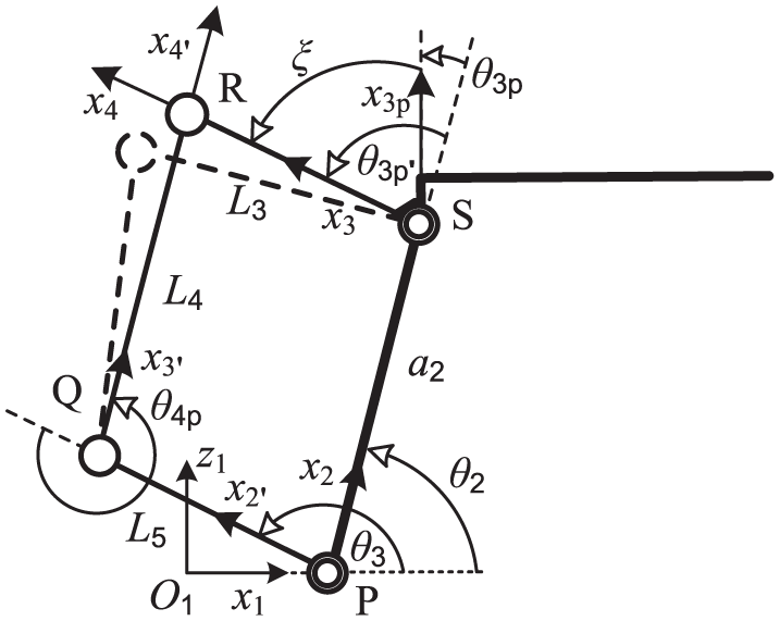
The closed-loop actuating mechanism PQRS of the HH800 robot (dashed lines represent a degenerated mechanism).
For simplicity, the closed-loop actuating mechanism PQRS can be considered as a planar mechanism. The position constraints for the closed loop are formed with respect to the plane O1x1z1 as follows28,29

where
The closed-loop PQRS is a parallelogram, and therefore it has properties such as
It is worth to mentioning that when the closed mechanism degenerates (dashed line in Figure 2), its actual link lengths differ from its nominal values. The passive joint position can be computed by
Because the robot kinematic model in equation (2) is used for calibration, a modification of a link transformation is required if two joint axes of this link are parallel (or nearly parallel). This transformation is modified as in the research
4
to satisfy the properties of the calibration robot model: complete, proportional, and continuous.
23
Particularly, the transformation matrix

where
Robot joint compliance model
In a robot static configuration, a robot joint torque causes a twist deformation about a rotation shaft (which represents the entire drive train from the motor to the associated robot link). We can consider the shaft as a torsion spring.
In this section, we study characteristics of a torsion spring because they are related to modeling of rotational joint compliance. The characteristics of torsion springs are basically presented by non-linear functions, for example, M = k(δθ)3, where M is the applied torque on the spring, δθ is the spring rotational deformation, and k is the torsion spring’s stiffness parameter (p. 335). 27 Because the robot joint deformation is small, we can assume that the functional relationship between the joint torque and its deformation is linear. This work is the extension to closed chain manipulator for the previous work. 10
The model of robot joint deformation, which is caused by the joint torque, can be represented by

where Mi (Nm) is the joint torque applied at joint axis i, ki (Nm/rad) is the stiffness parameter of joint i, si (rad/Nm) is the compliance parameter (it is the inverse ratio of the joint stiffness parameter) of joint i, and δθi (°) is the deformation angle of joint i under applied torque Mi,
For serial robots with one closed-loop mechanism such as the Hyundai HH800 robot, the active joint torques are computed by following the methods presented in the studies.29,30
In order to compute the robot joint torques of active joints, we applied a virtual work principle and a technique for analyzing the original robot to form an open tree-structure robot. By assuming that the joint R of the closed-loop PQRS (Figures 1 and 2) is cut open, we can obtain an open tree-structure mechanism that consists of two open chains. The first chain is connected by the joints
In this section, we built the robot kinematic model consisting of geometric and joint compliance parameters. The next section presents a formulation for the identification of these parameters.
Formulation for parameter identification
The robot calibration process identifies robot kinematic model parameters that describe exactly the kinematics of a physical robot and consequently enhance the robot position accuracy. This section describes robot kinematic parameter identification. A robot kinematic model consists of link geometric and joint compliance parameters.
Because the robot consists of a main open chain and a closed-loop mechanism (Figure 1), in order to identify the kinematic parameters of the entire robot kinematic model, robot identification equations are formulated by integrating the differential equations of the open chain and the closed loop via the passive joint angle
Differential transformation of the open kinematic chain can be obtained by differentiating equation (2) in terms of its kinematic parameters as follows 5

where
where
The position constraints (5) of the closed-loop PQRS (Figure 2) can be expressed in the following form

By differentiating the variable

By the expansion of equation (8), we have the following equation

The identification equation of kinematic parameter errors (of the open chain and the closed loop) can be obtained by integrating equation (11) into equation (12) via the passive joint parameter

where column vectors

Equation (13) describes the differential relationship between robot geometric errors and its end-effector position errors. In order to take into account the effects of its joint compliance errors, the identification equation (13) has to be modified as follows

where a Jacobian matrix

where
Substituting equation (16) into equation (15), after some manipulations we obtain the identification equation of the robot kinematic errors, which comprises the geometric errors and joint compliance parameters
The robot model that is used for the calibration includes many kinematic parameters. Only some of them, however, are identifiable. In order to determine the identifiability of the parameters, a technique from the previous study 31 is applied. This technique uses two measures, mag(pi) and var(pi), which are based on the singular value decomposition of the identification matrix J, where pi is the ith robot parameter. Among the 30 parameters of the robot open kinematic chain that are listed in Table 2, d2 and d6 are the coupling parameters of d3 and d7, respectively; a6 and b7 are the coupling parameters of θ6. For the robot closed-loop mechanism, it is necessary to fix one length parameter (L3 is selected to be fixed) to scale the size of the mechanism. 30 The coupling parameters cannot be determined together. The sign “×” in Table 2 indicates the indeterminable parameters. Thus, only 29 kinematic parameters of the HH800 robot are observable (n = 29).
Identified D-H parameters of HH800 robot (units: length (m) angle (°) “–”: unavailable, “×”: un-identifiable).
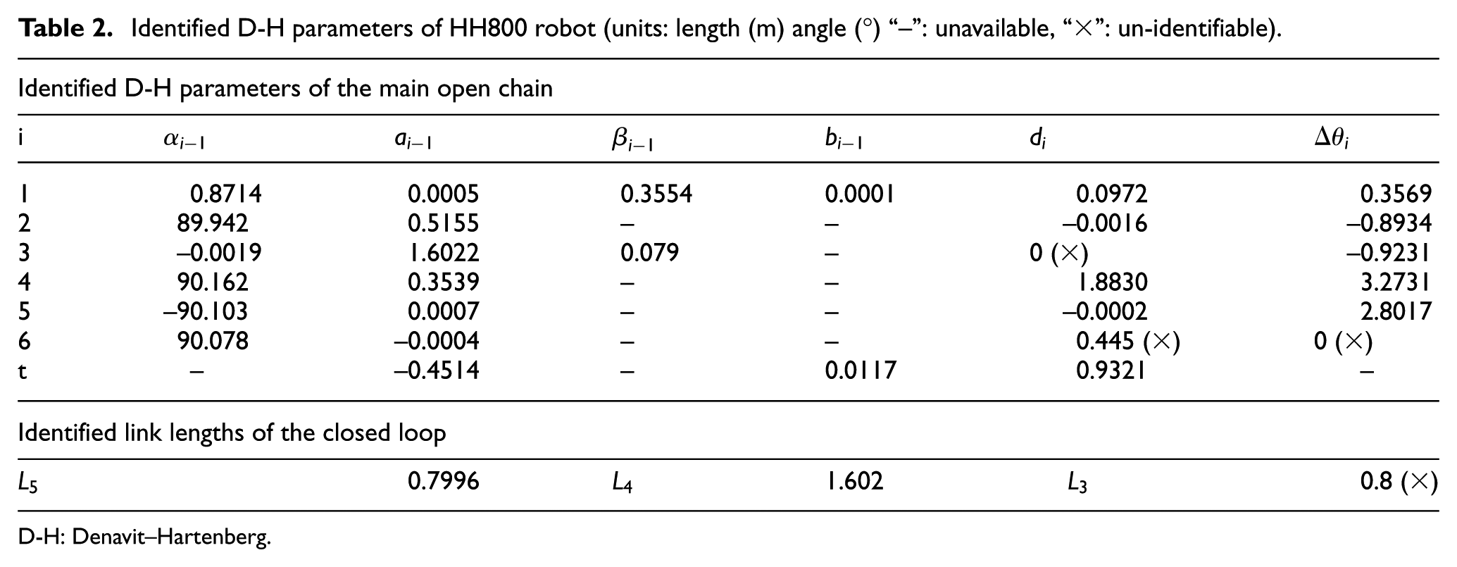
D-H: Denavit–Hartenberg.
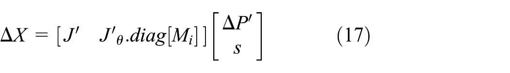
The robot end-effector position errors are caused by many kinematic error sources, which can be classified into geometric and non-geometric errors. Equation (17) is utilized for identifying the robot geometric errors and partial non-geometric error (joint compliance errors due to the effect of gravity of the robot link and payload). However, other non-geometric error sources such as gear backlash and link deflection should be taken into account because they also affect the robot position accuracy. It is very difficult to model all the non-geometric errors completely and exactly. Therefore, the residual position errors after geometric and joint compliance correction should be compensated for by using an ANN. Application of the ANN for further enhancing robot accuracy is presented in the next section.
ANN and its application for robot position error compensation
The robot position errors after correction using the identified link geometric and joint compliance errors are still large. The residual position errors are supposed to be caused by undetermined non-geometric error sources, which have extreme non-linearity. 32 In order to increase the robot accuracy, an ANN will be used to compensate for the residual position errors.
In this study, an ANN that has three layers is constructed as in Figure 3. The input layer consists of six nodes. These nodes represent six robot joint positions [θi],

Construction of a three-layer ANN.
The ANN needs to be trained prior to applying for non-geometric error compensation. A back-propagation algorithm is used to train the ANN.33,34 The training data include pairs of input and output values. The inputs are robot joint encoder readings. The outputs are the residual position errors after correction of the robot geometric and joint angle deflection errors.
Equation (15) describes the relation between the robot end-effector position errors and its kinematic errors (geometric errors and joint compliance parameters). This equation should be manipulated suitably into equation (17) for identifying the vector of the joint compliance parameter
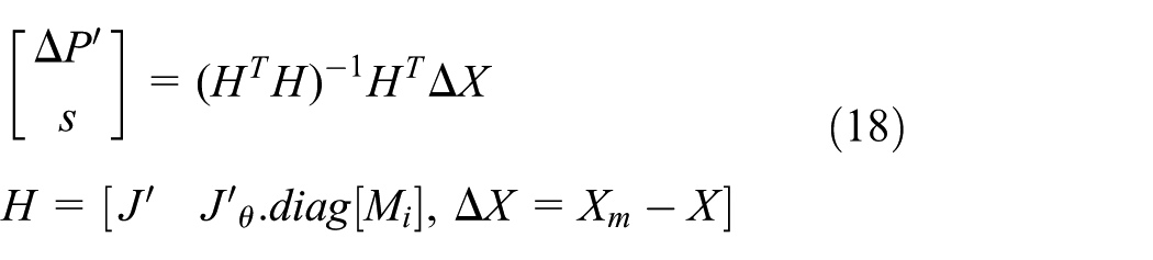
where Xm is a (3 × 1) vector of the end-effector position measurement. X is a (3 × 1) vector of the end-effector position that is computed with the current robot kinematic parameters.

where
The correction process for the robot position is depicted by a flowchart as in Figure 4. First, the robot link geometry and joint compliance errors are identified simultaneously by equation (18). After that the residual robot position errors after compensation for link geometry and joint compliance errors are used for training the ANN. The residual position errors are supposedly caused by other un-modeled non-geometric error sources such as robot link deformation and gear backlash. The modified robot model and the trained ANN are used to compute the robot end-effector positions for a given robot joint position reading.

A methodology for robot end-effector positioning.
There are many methods of compensation for robot position error. Among them is a so-called “false target” technique, 15 which is used widely for robot OLP. The OLP contains a set of modified robot joint commands, which is used to guide the robot to its desired position in the workspace with a specific accuracy. The readers can see more details in the work, 15 which presented many compensation methods for robot position errors.
Experiment and results
The proposed method is applied for the experimental calibration of a Hyundai HH800 robotic manipulator. The enhanced position accuracy of the robot after calibration proves the effectiveness and correctness of the proposed method. This section presents orderly steps of experimental calibration such as arrangement of the robot calibration system, measurement process, calibration results, and validation of robot accuracy after calibration.
A robot calibration system consists of a Hyundai HH800 robot (6 dof), which has one closed-loop actuating mechanism, a three-dimensional (3D) point sensing device (API Laser Tracker, measurement accuracy of 0.01 mm/m, repeatability of ±0.006 mm/m), and an accompanying laser reflector. The reflector is fixed at a particular location of the robot end-effector. The system is arranged as shown in Figure 5.
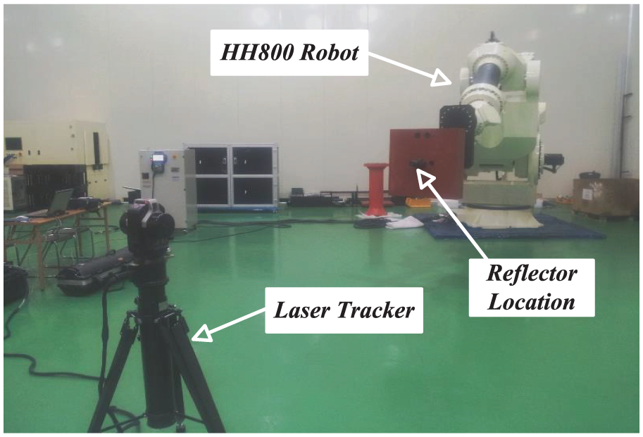
Calibration setup of the Hyundai HH800 robot.
In order to acquire suitable measurement data for robot parameter identification and ANN training, the robot workspace is divided into 10 sub-workspaces which are depicted in Figure 6. In each sub-workspace (the central angle is 18°), the robot moves its end-effector to 50 positions such that they entirely cover the sub-workspace. The 3D coordinates of the end-points are measured by the Laser Tracker and saved in a computer. At the same time, the associated robot joint readings also are recorded. For the other sub-workspaces, the measurement procedure is performed similarly. As a result, a set of 500 end-effector positions and a set of 500 robot joint angle readings are acquired. These measurements will be grouped as follows: a set of 4 × 10 = 40 end-effector positions (referred to as Q1) for parameter identification is collected from the sub-workspaces (4 end-points from each of 10 sub-workspaces).
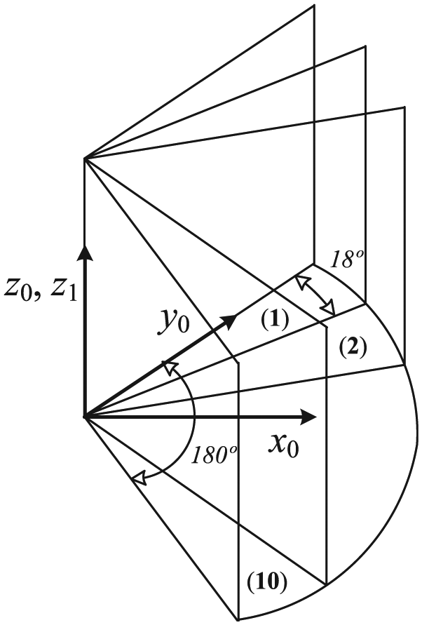
An arrangement for collecting robot end-effector measurements in each sub-workspace.
A set of 20 × 10 = 200 (referred to as Q2) robot end-points for training the ANN is collected from the sub-workspaces (20 end-points from each of 10 sub-workspaces). A set of 20 × 10 = 200 (referred to as Q3) arbitrary end-points for robot accuracy validation is collected from the sub-workspaces (20 end-points from each of 10 sub-workspaces).
Elements of the sets Q1 and Q2 should be totally different. It is worth to noting that the sets Q1 and Q2 of end-points are selected such that these points have a uniform distribution within each sub-workspace.
In the identification process, we first identify the robot link geometric errors and joint compliance parameters by using the measurement set Q1. By using the whole set Q1, we can define an overdetermined system of 120 (3 × 40 = 120) differential equations based on equation (17). The solution (equation (18)) of this system of equations in the sense of least squares is identified link geometry and joint compliance parameters. 35 The total number of identifiable parameters is 29 (25 geometric parameters and 4 joint compliance parameters, s2, s3, s4, and s5). With this type of robot, the first joint axis is vertical, so the s1 parameter is not taken into account because the torsional deformation about the first axis is so small compared with other joint axes. The joint deformation about the sixth axis is not identifiable because of dependence characteristics associated with other parameters. 31 The identified values of these geometric parameters are listed in Table 2. The compliance parameters of joints 2, 3, 4, and 5 are s2 = (1/2.348) × 10−7 (rad/Nm), s3 = (1/5.702) × 10−6 (rad/Nm), s4 = (1/1.728) × 10−6 (rad/Nm), and s5 = (1/2.074) × 10−6 (rad/Nm), respectively.
After compensating for the robot link geometry and joint compliance errors, the residual end-effector position errors are still fairly large. The residual errors are supposedly caused by the other non-geometric error sources (e.g. the robot link deformation, gear backlash). In order to reduce the residual position errors, the ANN is applied to compensate for these robot non-geometric error sources. Because the set Q2 is used for training the ANN, and in order to prepare the training data, the residual position errors are computed for a total of 200 positions of the set Q2. The position errors are displayed in Figure 7. This figure shows the residual robot end-effector position errors after geometry and joint compliance error compensation. The ANN should be trained before it is used for error compensation.

The residual position errors after correction of geometric and joint compliance error (being used as ANN training output data).
The ANN is trained by the data that consist of the robot joint readings Q2 (the ANN training input) and the residual position errors (the ANN training output as shown in Figure 7). As a result, after non-geometric error compensation using the trained ANN, the average robot position accuracy is enhanced drastically up to 0.3264 (mm) from 4.0654 (mm) (before calibration). The more details are shown in Tables 3 and 4. The residual position errors at measurement points are displayed in Figure 8. A portion of Figure 8 is magnified and is then displayed in Figure 9 for better presentation.
Absolute position accuracy of the HH800 robot (calibration).
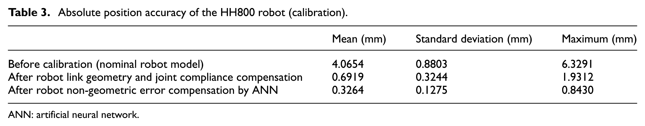
ANN: artificial neural network.
Absolute position accuracy of the HH800 robot (validation).

ANN: artificial neural network.
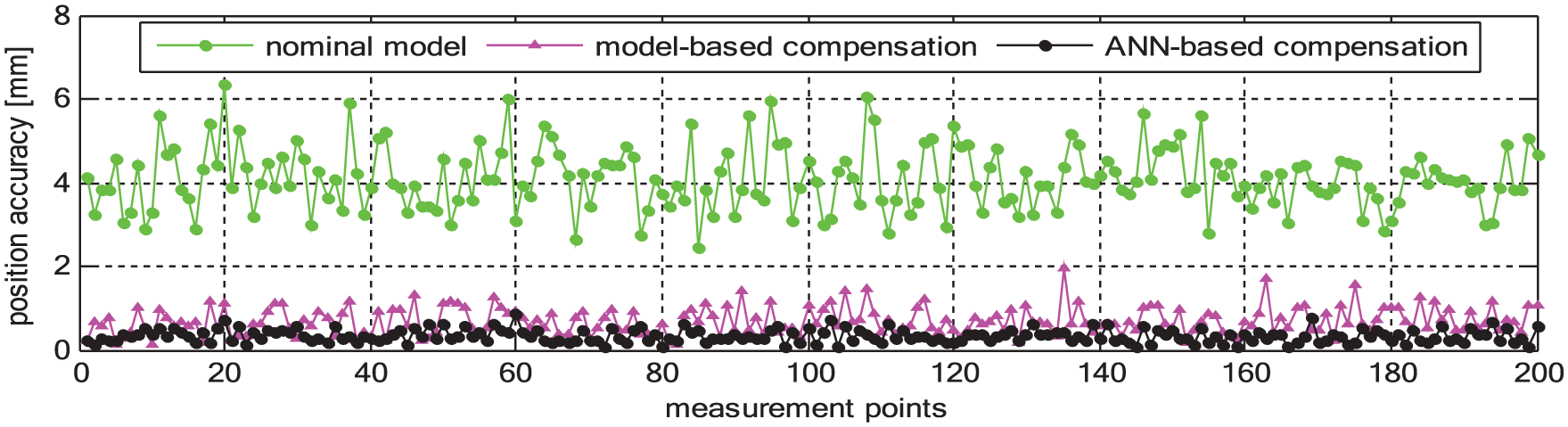
Absolute position accuracy of the HH800 robot (before and after calibration).

Magnification of a section of Figure 8.
The robot position accuracy at the calibration measurement points is normally higher than the accuracy at other arbitrary measurement points. In this section, a validation of the robot performance after calibration is performed with the measurement set Q3 (mentioned above). The validation results show that the robot average position accuracy after link geometry and joint compliance error correction is 0.7035 (mm), maximum position error is 2.1372 (mm), and after non-geometric error compensation by the ANN is 0.3959 (mm) (maximum position error is 0.8928 (mm)).
The position errors at measurement points are also shown in Figure 10. The position errors for the validation data set Q3 (in Figure 10) have the same order of magnitude as those of the calibration data set Q2 (in Figure 9). Therefore, the robot after calibration has the same level of position accuracy across the data set Q2.

Absolute position accuracy of HH800 robot (validation).
Conclusion
This article proposed a new calibration method for enhancing robot position accuracy. The method is a combination of a model-based calibration procedure and an ANN-based error compensation technique. The model-based calibration method has many advantages such as less computing time, fast convergence, and accurate knowledge of error sources. Some error sources (especially non-geometric errors) cannot, however, be determined and modeled correctly. Therefore, in order to further increase the robot position accuracy, the un-modeled error sources should be compensated for by using an ANN.
The experimental calibration was performed on the Hyundai HH800 robot. After calibration, the robot average accuracy is increased significantly to 0.3264 (mm) (from 4.0654 (mm) before calibration). The calibration results demonstrate the effectiveness and correctness of the proposed method. In addition, the validation results for robot accuracy at arbitrary points show that the robot after calibration has the same level of position accuracy in its entire workspace.
Footnotes
Handling Editor: Guanglei Wu
Declaration of conflicting interests
The author(s) declared no potential conflicts of interest with respect to the research, authorship, and/or publication of this article.
Funding
The author(s) disclosed receipt of the following financial support for the research, authorship, and/or publication of this article: This research was supported by Basic Science Research Program through the National Research Foundation of Korea (NRF) funded by the Ministry of Education (NRF-2016R1D1A3B03930496).