Sage Journals: Discover world-class research

Abstract

A pipeline operation optimization model with minimum energy consumption as the objective function was established based on the dynamic programming method. The model was applied to a 3840 km gas pipeline whose designed pipeline capacity was 170 × 10⁸ t/a. There were 40 stations in the line, including 22 compressor stations and 32 compressors. The solution time was controlled within 60 s to show that the algorithm was fast and effective. The number of starting-up compressors in the optimized scheme is two more than that in the actual operation scheme, and the total pressure drop of the pipeline decreased by 3.40 MPa, the average efficiency of the gas turbine units increased by 4.234%, the average efficiency of the electric drive units increased by 4.875%, and the power decreased by 18,720.38 kW, confirming the validity and feasibility of the optimization model.

Keywords

Dynamic programming energy consumption gas pipeline operation optimization

Introduction

The goal of gas transmission pipeline operation optimization is to minimize the energy consumption and flow noise of the pipeline system and maximize the pipeline throughput. However, this is very difficult to achieve, because more gas requires higher pressure and more compressor energy consumption and creates greater flow noise.^1,2,3 For a long gas pipeline, the main expense is the running cost of the compressor stations. Studies have shown that the energy consumption of the compressors is more than 50% of the total energy consumption of a pipeline.^4,5 However, optimization methods can be used to direct the operation of compressor stations so that the economy of this part is improved, lowering the cost of the entire pipeline system and maximizing the gas pipeline filling on the premise of safety.

In the 1960s, the United States and some countries in Europe began research on optimizing the operation of gas transmission pipelines. The original mathematical models were steady state, taking the lowest energy consumption of a compressor as the objective function, and the optimal operation plan of compressors was determined through a set of optimization calculations. PJ Wong and RE Larson⁶ started the use of dynamic programming in 1968 to solve the modeling of gas pipeline operation optimization. Over the next decades, several studies on pipeline optimization modeling were done, both in China and in overseas.

Objective function: In pipeline optimization, the objective function is usually the maximum throughput,⁷ the maximum filling of the pipeline,^8,9 or the lowest pipeline energy consumption.^10,13 Of these, the latter is the most common focus. In this study, the operation conditions of a gas pipeline were optimized using the lowest energy consumption as the objective function.

Constraint condition: There are usually three kinds: inequality constraints, equality constraints, and compressor constraints. Inequality constraints are used to limit the flow, pressure, and temperature of a pipe within a specific range.¹¹ Equality constraints are governing equations of gas flow in the pipeline, including a mass conservation equation, a pressure equation, and a temperature equation.¹⁰ Compressor constraints were first established based on ideal compressor assumptions, which ignored the nonlinear relations between the pressure head, power, efficiency, compression ratio, and flow of a compressor. Wu et al.¹² and Liu et al.¹³ built up a set of polynomials including surge curves and stagnation curves to describe feasible regions that overcame the shortcomings of the ideal compressor model. Sanaye and Mahmoudimehr¹⁴ promoted their compressor constraints by considering correction parameters relevant to the ambient temperatures, component load running, and excess operations of compressors, which were more likely to represent actual compressor operation. In addition to the operation parameters of a compressor, the operation state (on or off) is also an essential parameter to be optimized, especially for a system with a set of compressors.¹⁵

Optimization variables: Optimization variables are arguments of an optimization model, which generally consist of pressure, temperature of each node, flow rate of each unit (pipe and compressor), and the running state and efficiency of each compressor. The pressure, temperature, and efficiency of a compressor are continuous, whereas the running state of a compressor is discrete.^16–18

Over the past decades, experts have promoted many algorithms to solve the pipeline optimization problem. Dynamic programming, generalized reduced gradient, and linear programming were the most common. But dynamic programming became the most successful algorithm for solving this kind of problem because of its advantages of ensuring global optimization and easy handling of nonlinear situations.^19–23

After years of effort by experts, many algorithms are now available to create natural gas pipeline optimization models, but research on and energy consumption models of gas pipelines with very large compressors based on dynamic programming is insufficient. In our research, based on the characteristics of long distances and multiple compressor stations, an optimal operating plan was determined that accommodated the actual conditions of a pipeline. By taking a gas pipeline as an example, we created a relevant dynamic programming optimization model whose results have shown its feasibility.

Modeling and method

Modeling

Objective function

Our objective function reflected the objectives of pipeline operations. In the actual situation, the lowest energy consumption is taken as the objective function, and because it consists mainly of the energy consumption of compressor stations, the objective function can be the minimum sum of that energy consumption

\min F = \sum_{i = 1}^{m} \sum_{j = 1}^{n} f_{i} (k_{ij}, Q_{ij}, P_{di})

(1)

where F is the total energy consumption of all compressor stations; f_i is the energy consumption of the ith compressor station, i = 1, 2, 3,…, m; k_ij is the switch state of the jth compressor in the ith compressor station, where k_ij = 0 means no power on, and k_ij = 1 means power on; Q_ij is the flow rate of the jth compressor in the ith compressor station in m³/s (it is divided evenly when the compressor configuration in the station is the same); and P_di is the outbound pressure of the ith compressor station in MPa.

Optimization variables

The outbound pressure and the running state of the compressors are directly related to the objective function of the optimization model. The energy consumption of a compressor depends on its compression ratio, flow rate, and temperature, but when the inlet condition of the compressor station is known, the energy consumption can be simplified as a function of compression ratio and temperature. The inlet and outlet temperatures of a compressor also depend on its compression ratio, so the optimization variables can be set to be the compression ratio that optimizes the outbound pressure. As a result, we set the optimization variables of the pipeline optimization model to be the number of powered-on compressors and the outbound pressure of a typical compressor station

X = (P_{di}, k_{ij})

(2)

Constraint conditions

To ensure the operation security of the pipeline and equipment, the process parameters must be restricted within a certain range that meets the constraint conditions of the model.

Flow rate constraints

The amount of gas can change in only a certain range, which is

Q_{i \min} ⩽ Q_{i} ⩽ Q_{i \max} (i = 1, 2, \dots, N_{n})

(3)

where Q_i is the intake (partial) volume of node i in m³/s, $Q_{i \min}$ is the minimum intake (partial) volume allowed by node i in m³/s, and $Q_{i \max}$ is the maximum intake (partial) volume allowed by node i in m³/s.

Node pressure constraints

The pressure of each natural gas pipeline node must be limited based on the terminal demands, thus

P_{i \min} ⩽ P_{i} ⩽ P_{i \max} (i = 1, 2, \dots, N_{n})

(4)

where P_i is the node i pressure in MPa, $P_{i \min}$ is the minimum pressure allowed by node i in MPa, and $P_{i \max}$ is the maximum pressure allowed by node i in MPa.

Pipe stress constraints

When there are N_p pipes in the gas pipeline system, for the sake of pipeline safety, the pressure in pipe k must be less than the maximum allowable operating pressure, which is

P_{k} ⩽ P_{k \max} (k = 1, 2, \dots, N_{p})

(5)

where P_k is the pressure of natural gas in pipeline k in MPa, and $P_{k \max}$ is the maximum pressure allowed in pipeline k in MPa.

Flow equilibrium constraints

Because of the conservation of mass, for each pipe node, the gas mass flow into and out of the node should be consistent. Generally, for a gas pipeline system with Nn nodes, the gas flow balance equation of nodes can be written as

\sum_{\binom{k \in C_{i}}{i = 1}}^{Nn} α_{ik} M_{ik} + Q_{i} = 0

(6)

where C_i is a collection of components connected to node i, M_ik is the absolute value of the flow in (or out) from the ith node of the connected component k, Q_i is the flow exchanged between node i and the outside world (inflow is positive and outflow is negative), and α_ik is the coefficient (when the flow from k components flows into the i node, it is +1; when it flows out of the i node, it is −1).

Compressor performance constraints

The compressor power equation is

N = \frac{MH}{η}

(7)

where M is the overflow rate of the compressor in kg/s, H is the polytropic head of the compressor, and η is the efficiency of the compressor.

The head curve is calculated according to

- H = h_{1} S^{2} + h_{2} SQ + h_{3} Q^{2}

(8)

where h₁, h₂, and h₃ are the fitting coefficients of the head curve, S is the speed of the compressor, and Q is the actual overflow rate of the compressor in m³/d.

The efficiency curve is calculated according to

\frac{- H}{η} = e_{1} S^{2} + e_{2} SQ

(9)

where $e_{1}$ and $e_{2}$ are the fitting coefficients of the power curve.

The buzz curve is calculated according to

Q_{surge} = s_{1} + s_{2} H

(10)

where Q_surge is the surging flow in m³/d, and s₁ and s₂ are the fitting coefficients of the buzz curve.

The stagnation curve is calculated according to

Q_{stone} = s_{3} + s_{4} H

(11)

where Q_stone is the stagnation flow in m³/d, and $s_{3}$ and $s_{4}$ are the fitting coefficients of the stagnation curve.

Equations (7)–(11) are plotted in Figure 1, forming a closed area. This area is the operating area of the compressor. Using the online test software of the Beijing Oil & Gas Pipeline Control Center, we obtained the actual running data of the compressor in real time, and then corrected and fitted the curve of the compressor to obtain the actual running of the compressor curve (Figure 1), which had rarely been considered before.

Figure 1.

Compressor head characteristic curve.

Compressor power constraints

The power of every compressor (station) was limited to the characteristics of the compressor

N_{j \min} ⩽ N_{j} ⩽ N_{j \max} (j = 1, 2, \dots, N_{c})

(12)

where N_j is the power of the jth compressor (station) in W, $N_{j \min}$ is the minimum power of the jth compressor (station) allowed in W, and $N_{j \max}$ is the maximum power of the jth compressor (station) allowed in W.

Outlet temperature constraints

The outlet temperature of every compressor was restricted

T_{d} ⩽ T_{d max}

(13)

where $T_{d max}$ is the maximum outbound temperature of compressor station (K).

Method for modeling based on dynamic programming

Dynamic programming is one of the most important solutions to pipeline optimization. It developed quickly with improvements in computer science. In this study, dynamic programming was innovatively applied to long-distance natural gas transmission pipeline operation optimization, which had not been done in previous studies.

Dynamic programming

When the distribution branch pipes along a gas pipeline are simplified to discharge nodes, the operation of the pipeline can be regarded as a multistage process; hence, dynamic programming is eligible for optimizing compressor stations along the pipeline, as shown in Figure 2.

Figure 2.

Schematic of dynamic programming stage.

We established the dynamic programming model of the optimal configuration of each compressor station in the pipeline as equations (14)–(22) after setting the number of compressors as m and considering the gas transmission process between the compressor station k – 1 and station k as stage k of the problem. In that problem, the state variable x_k (for the starting state of the phase) was the outbound pressure $(P_{d, k - 1})$ $(k ⩾ 2)$ of station k – 1, and the stage effect V_k was the energy consumption of station k. Taking the total energy consumption of the pipeline as the optimization objective, the dynamic programming model for the operation optimization of each compressor station of the pipeline can be established:

Stage variables

x_{k} = P_{d, k - 1}, k = 2 ~ m + 1

(14)

Decision variables

d_{k} = ε_{k}, k = 1 ~ m

(15)

Stage evolution equation

x_{k + 1} = T_{k} (x_{k}, d_{k}), k = 1 ~ m

(16)

Stage effect

V_{k} = C_{k} (x_{k + 1}, d_{k}), k = 1 ~ m

(17)

Objective function

V_{1, k} [x_{k + 1}, P_{1, k} (x_{k + 1})] = \sum_{i = 1}^{k} C_{i} (x_{i + 1}, d_{i}), k = 1 ~ m

(18)

Optimal objective function

f_{k} (x_{k + 1}) = \min_{P_{1, k} (x_{k + 1})} V_{1, k} [x_{k + 1}, P_{1, k} (x_{k + 1})], k = 1 ~ m

(19)

Function recurrence equation

f_{k} (x_{k + 1}) = \min_{d_{k} \in D_{k}^{γ} (x_{k + 1})} {f_{k - 1} (x_{k}) + C_{k} (x_{k + 1}, d_{k})}, k = 1 ~ m

(20)

Initial conditions

x_{1} = P_{d, 0} (Supply pressure of gas source)

(21)

and

f_{0} (x_{1}) = 0

(22)

where $P_{d, k}$ is the outbound pressure at the kth station and $D_{k}^{γ} (x_{k + 1})$ is the kth phase corresponding to the allowed decision set of its endpoint state x_k_+ 1.

Solution

The solution to dynamic programming applied to the pipeline optimization model comprises four main parts: (1) state space determination, (2) recurrence between stations, (3) recurrence within stations, and (4) a backtracking algorithm, as shown in Figure 3.

Figure 3.

Flowchart of the pipeline operation optimization dynamic programming algorithm.

Case study

Operation program optimization

The total length of the west–east gas pipeline we studied was 3840 km. The designed pipeline capacity was 170 × 10⁸ t/a and the pipe diameter was 1016 mm. The pipe length between each compressor station and the number of compressors in each station are shown in Figure 4.

Figure 4.

Length of pipe between each compressor station and number of compressors in each station.

In this study, the curves for pressure head, pressure head/efficiency, surge flow, stagnation flow, speed, and flows of centrifugal compressors were fitted with actual field operation data. The centrifugal compressors of stations 13, 15, 16, 17, and 19 were selected for fitting calculation. The coefficient values in equations (8)–(11) are shown in Table 1.

Table 1.

Compressor characteristic curve coefficients.

Station number	h ₁	h ₂	h ₃	e ₁	e ₂	s ₁	s ₂	s ₃	s ₄
13	−0.000458	−0.000341	0.000067	−0.001470	0.000150	5630	0.387	10,100	1.36
15	−0.001190	0.000161	0.000042	−0.001450	0.000317	3610	0.149	4640	0.554
16	−0.000458	−0.000341	0.000067	−0.001470	0.000150	5630	0.387	10,100	1.36
17	−0.000597	0.000079	0.000008	−0.000701	0.000119	5050	0.481	8510	1.59
19	−0.000529	−0.000362	0.000129	−0.001260	0.000213	3340	0.265	6020	0.84

The daily operation report of a pipeline is the practical operation plan that can be acquired from the production daily report. Basing our work on the daily operation report of the west–east gas pipeline, to evaluate the effectiveness of the model, we generated the optimum operation programs and compared them with the appointed programs in the daily report. The transporting conditions and the injection and distribution volume of each station were demonstrated. As shown in Figure 5, there were 5 stations with gas injection and 20 stations distributing gas from the main stream to branches. The first station’s pitted temperature was 15°C and pitted pressure was 6.5 MPa.

Figure 5.

Multipoint injection volume and distribution volume.

Daily operation report (the practical operation program)

We obtained the process parameters of each station in the case from the practical operation report, as shown in Table 2.

Table 2.

Daily operation report of each compressor station in the case.

Stationnumber	Number of starting-upcompressors	Pittedpressure(MPa)	Outboundpressure(MPa)	Pittedtemperature (°C)	Outboundtemperature (°C)	Driving type	Unitefficiency (%)	Power(kW)
1	2	6.50	9.60	15.00	50.00	Gas turbine	18.5	22,085.62
2	1	7.40	9.60	8.25	46.40	Gas turbine	20.9	12,154.72
3	1	8.01	9.60	11.19	36.02	Gas turbine	20.3	6227.12
4	1	7.79	9.60	7.32	47.71	Gas turbine	20.5	9640.90
5	1	7.44	9.60	8.75	39.66	Gas turbine	17.7	13,732.41
6	1	8.30	9.60	10.20	32.82	Gas turbine	19.8	4867.49
7	1	7.37	9.60	8.53	32.86	Gas turbine	20.0	12,602.96
8	1	8.04	9.60	8.13	37.22	Gas turbine	20.3	8068.03
9	1	7.56	9.60	8.71	31.16	Gas turbine	17.5	6431.34
9	1	7.56	9.60	8.71	31.16	Motor	55.0	6431.34
10	1	7.74	9.54	6.70	45.68	Gas turbine	20.7	9360.03
11	1	7.57	9.60	10.48	35.05	Gas turbine	19.6	11,469.92
12	0	8.54	8.54	11.91	11.91	Gas turbine	0	0
13	1	7.03	9.60	6.20	28.52	Gas turbine	23.7	12,407.30
15	1	8.38	9.50	7.28	36.59	Gas turbine	22.3	4778.48
16	2	6.17	9.61	8.48	38.31	Gas turbine	23.5	22,190.25
17	1	7.67	9.69	13.25	36.34	Gas turbine	23.5	11,277.80
19	1	7.52	9.62	11.27	38.88	Gas turbine	23.5	11,666.51
20	1	7.34	9.10	12.53	36.29	Motor	59.3	12,855.52
22	1	6.36	9.23	10.85	36.27	Gas turbine	23.9	17,920.78
24	1	6.84	9.42	10.46	46.94	Motor	72.9	14,806.21
26	1	7.20	9.29	9.70	29.65	Motor	75.1	9299.43
29	1	5.93	8.23	5.42	24.38	Gas turbine	23.5	11,652.61

As shown in Table 2, in the actual operation scheme, the total number of starting stations of the compressors was 23—at least one for every station listed, except for compressor station 12. All the other compressor stations were in the starting state, of which only stations 1 and 16 opened two compressors. For a compressor station driven by a gas turbine, unit efficiency refers to the combined efficiency of the gas turbine and the compressor. For a compressor station driven by a motor, unit efficiency refers to the combined efficiency of the electric drive and the compressor. The average efficiency of a gas turbine unit was 21.09%, the average efficiency of a motor-driven unit was 65.58%, the total pressure drop was 44.67 MPa, and the total power was 245,495.4 kW. In actual operation, the energy consumption was high, the pressure drop was large, the unit efficiency was low, and there was still much room for optimization.

Optimized operation program

After calculations, we obtained the optimum operation program shown in Table 3. In the optimum program, stations 4, 8, and 12 were powered off; for stations 3, 7, 10, 11, 15, 16, 17, 19, and 20, a total of nine stations, outbound pressures were all 9.8 MPa, which was the design pressure of the pipeline.

Table 3.

Optimized operation scheme of the case.

Stationnumber	Number ofstarting-upcompressors	Pittedpressure(MPa)	Outboundpressure(MPa)	Pitted temperature (°C)	Outbound temperature (°C)	Drivingtype	Unitefficiency (%)	Power(kW)
1	1	6.50	9.08	15.00	43.92	Gas turbine	23.7	15,356.19
2	2	6.72	9.43	7.72	36.25	Gas turbine	23.5	15,144.34
3	1	7.86	9.80	9.69	28.14	Gas turbine	23.9	9291.68
4	0	8.14	8.14	6.78	6.78	Gas turbine	–	–
5	2	5.68	9.41	5.15	48.17	Gas turbine	23.7	23,151.83
6	1	8.07	9.46	11.12	24.34	Gas turbine	23.5	6782.50
7	2	7.29	9.80	7.40	32.21	Gas turbine	23.5	12,900.89
8	0	8.37	8.37	8.00	8.00	Gas turbine	–	–
9	2	6.17	9.15	5.32	38.56	Gas turbine	23.5	8852.01
9	2	6.17	9.15	5.32	38.56	Motor	74.0	8852.01
10	2	7.19	9.80	6.91	32.84	Gas turbine	23.6	13,620.97
11	1	8.00	9.80	8.78	25.73	Gas turbine	18.9	10,749.27
12	0	8.87	8.87	9.76	9.76	Gas turbine	–	–
13	1	7.45	9.32	5.81	24.31	Gas turbine	23.6	9438.34
15	1	8.15	9.80	6.73	21.95	Gas turbine	23.2	9310.21
16	2	6.94	9.80	6.91	35.96	Gas turbine	23.5	18,081.05
17	1	8.07	9.80	12.50	28.93	Gas turbine	23.2	10,192.83
19	1	7.92	9.80	9.68	27.47	Gas turbine	23.4	10,817.19
20	1	7.83	9.80	9.94	28.73	Motor	61.9	13,790.17
22	1	7.63	9.59	9.48	28.71	Gas turbine	23.7	11,545.28
24	1	7.71	9.43	9.11	25.88	Motor	70.8	10,087.37
26	1	7.58	9.49	7.26	25.90	Motor	75.1	8934.04
29	1	6.67	8.34	5.31	23.72	Gas turbine	23.1	8728.89

Number of starting-up compressors, Power of compressor units, pitted and outbound pressure of each station, pressure drop along the pipeline, average efficiency of the driving device are compared in the daily operation report and the optimized operation scheme, as shown in Figures 6 –10.

Figure 6.

Comparison of the numbers of starting-up compressors.

Figure 7.

Power comparison between actual operation and optimized operation.

Figure 8.

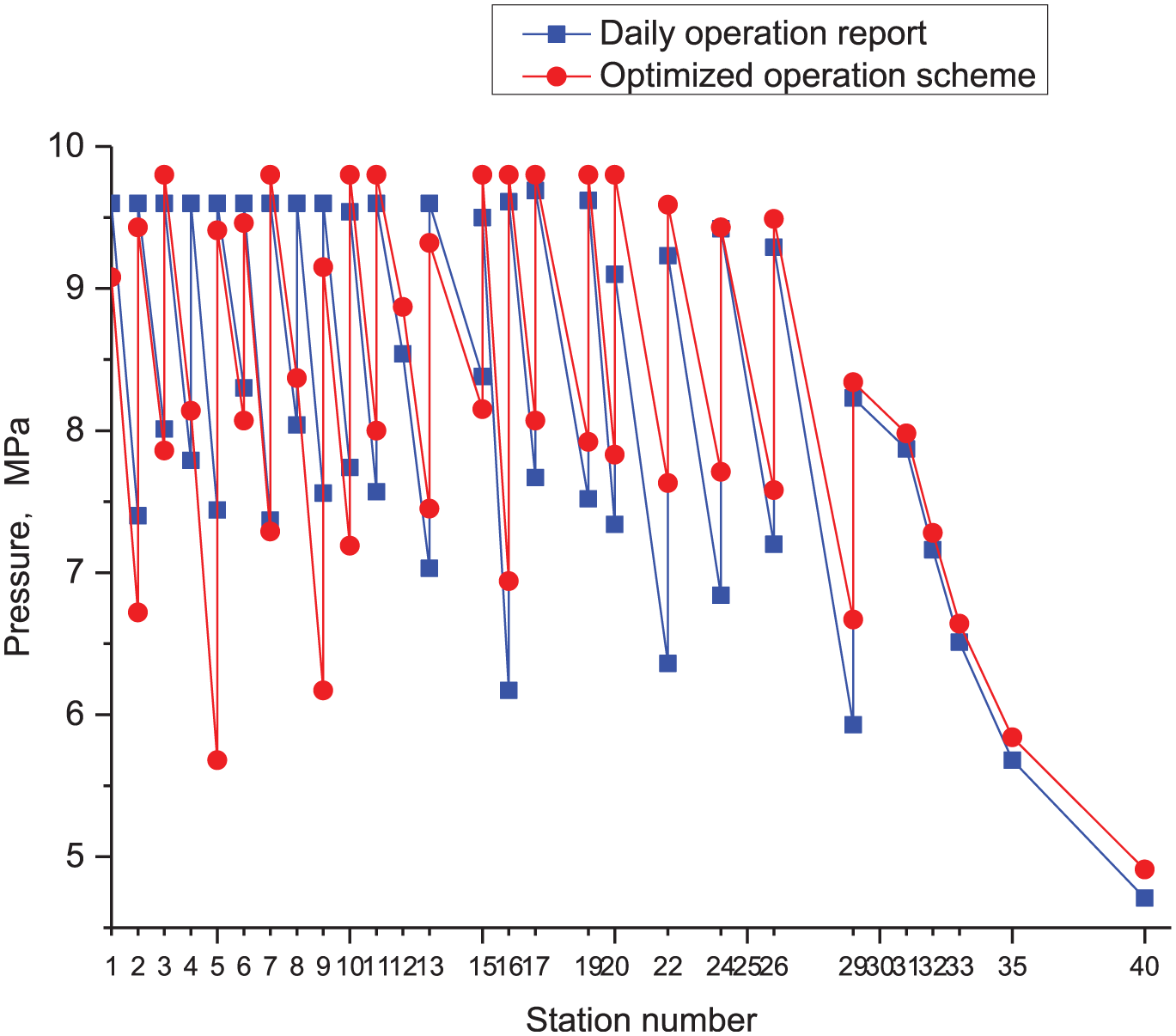
Comparison of inlet and outlet pressures.

Figure 9.

Comparison of pressure drops between daily operation report and optimized operation scheme.

Figure 10.

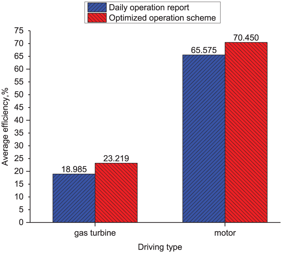
Comparison of average efficiency between daily operation report and optimization operation scheme.

In the actual operation scheme, there were 23 starting-up compressors. In the optimization operation scheme, there were 25 starting-up compressors: one compressor was added to stations 2, 5, 7, 9, and 10, and one compressor was removed from stations 1, 4, and 8.

According to the daily operation report, the total power used was 245,495.4 kW, and the total power used in the optimization scheme was 226,775.1 kW. The optimization scheme reduced the power used by 18,720.3 kW, or 7.6%. The power used by stations 1, 4, 8, 13, 16, 22, 24, and 29 decreased substantially, and the optimization results were obvious.

After optimization, the outbound pressures of stations 1, 3, 5, 6, 9, and 13 fell. In stations 4, 8, 11, 12, 13, 16, 17, 19, 20, 22, 24, 26, and 29, the pressures increased (the pitted pressure was low in station 5 because of a pressure crossing), thereby reducing the energy consumption of the compressors.

In the daily operation report, the total pressure drop of the pipeline was 46.46 MPa, whereas in the optimization plan, the total pressure drop of the pipeline was 43.06 MPa; the optimized scheme reduced the total pressure drop by 3.4MPa compared with the actual scheme. The pressure drops of pipeline sections 3, 7, 10, 11, 12, 15, 16, 17 + 18, 19, 20 + 21, 22 + 23, 24 + 25, and 26 + 27 + 28 decreased markedly.

After optimization, the efficiency of each station’s units was substantially improved. Except for station 11, the average efficiency of the gas-driven units was over 23%, and the average efficiency of the motor-driven units was over 70%. The average efficiency of the gas-driven units increased by 4.234% and that of the motor-driven units increased by 4.875%, which substantially reduced energy consumption.

As illustrated in the comparison charts above, the optimization program optimized the number of starting-up compressors at some compressor stations, the inlet and outlet pressures of stations, and so forth. The average pressure between stations was higher, and the pressure drop of most pipeline section was less. The total pressure drop in the actual operation scheme is 46.46MPa, and the total pressure drop in the optimized scheme is 43.06MPa. The total pressure drop in the optimized scheme is significantly lower than that in the actual operation scheme, which proves the feasibility and validity of the model and the solution method.

Estimation and comparison of optimum energy consumption

To compare and analyze the energy consumption of the pipeline, equations (23) and (24) were adopted to calculate its energy and gas consumption, and equation (25) was adopted to convert that consumption into standard coal consumption. The results are shown in Figures 11 and 12.¹³

Figure 11.

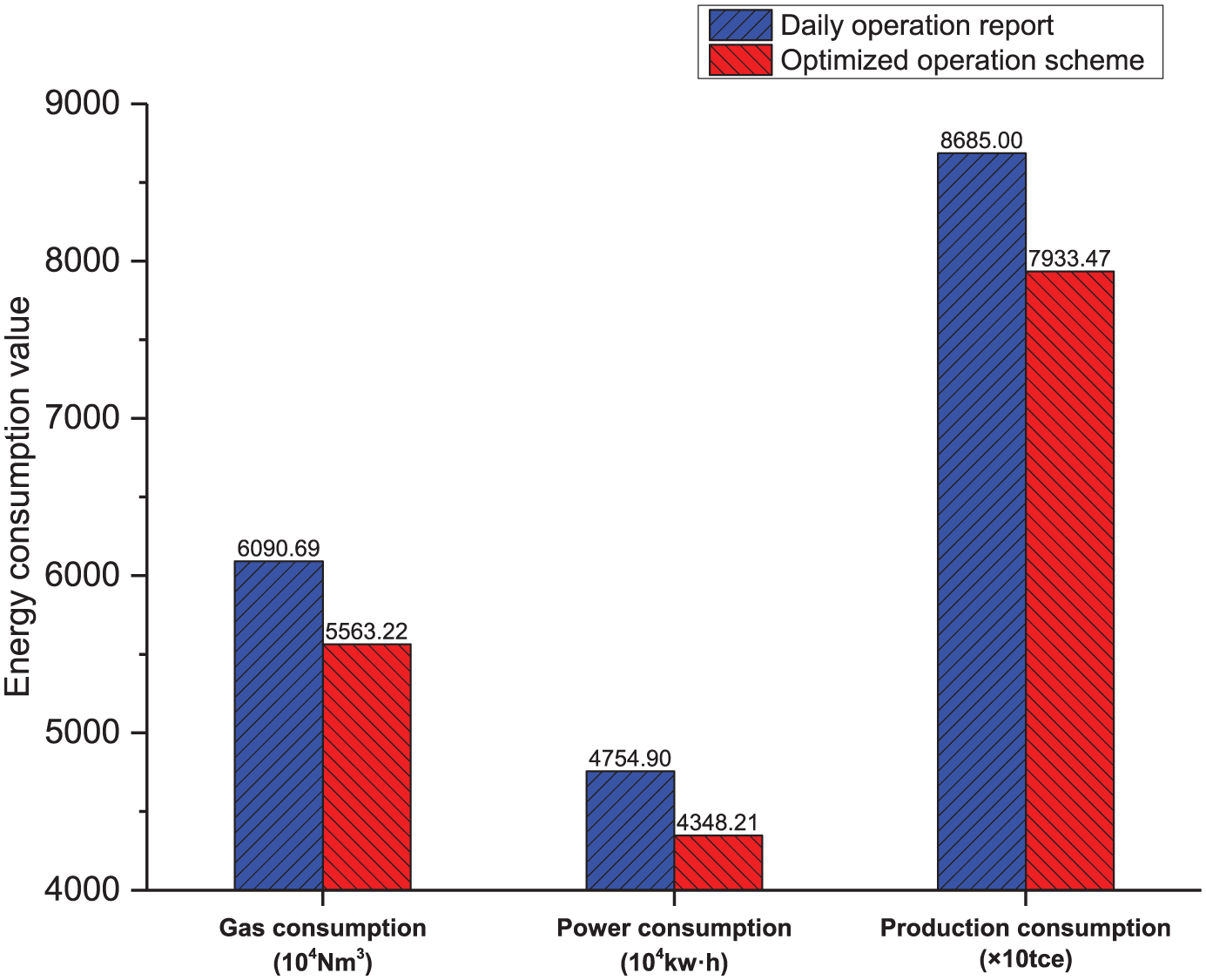
Comparison of total energy consumption.

Figure 12.

Comparison of unit energy consumption.

Based on the Chinese National Standard GB 52589-2008, the energy consumption of a pipeline is estimated by the indicators, such as gas consumption, power consumption, production consumption and gas unit consumption, power unit consumption, production unit consumption.

Gas consumption¹³ and power consumption are calculated by equations (23) and (24)

W_{g} = \sum_{i = 1}^{n} \frac{N_{i} t_{i}}{η_{gi}} ge

(23)

W_{e} = \sum_{i = 1}^{n} \frac{N_{i} t_{i}}{η_{ei}}

(24)

where W_e is the power consumption in kW·h, W_g is the gas consumption in m³, n is the number of compressors, $N_{i}$ is the shaft power of the ith compressor in kW, $t_{i}$ is the running time of the ith compressor in h, $η_{ei}$ is the drive motor efficiency of the ith compressor, is the turbine efficiency of the ith compressor, and ge is the gas loss rate of the gas turbine in N m³/(kW·h).

Hence, the total energy consumption is

F = \frac{W_{g} ω_{1} + W_{e} ω_{2}}{T_{ur}}

(25)

where F is the production unit consumption of the pipeline in kgce/(10⁷ N m³ ·km), $ω_{1}$ is the gas coal conversion coefficient based on the Chinese National Standard GB 2589-81 of 1.33 kgce/m³, $ω_{2}$ is the electric coal conversion coefficient based on GB 2589-81 of 0.1229 kgce/(kW·h), and T_ur is the turnover in 10⁷ N m³ ·km.

Figures 11 and 12 directly reflect that every energy consumption index was decreased after optimization, which confirms the feasibility and validity of the optimization model. Compared with the daily operation report, the optimization scheme reduced total gas consumption by 527.45 (10⁴ N m³), total electricity consumption by 406.69 (10⁴ kW·h), total production energy consumption by 7515.25 tce, and total energy consumption by 8.65%. Therefore, the optimized operation plan can save much energy.

Compared with the daily operation report, the optimization scheme reduced gas consumption by 11.39 (N m³/(10⁷ N m³·km), electricity consumption by 8.78 (kW·h/(10⁷ N m³·km), and production consumption by 16.24 (kgce/(10⁷ N m³·km)). The length of the west–east gas pipeline, the number of stations, the volume of transmission, and the number of compressors are large. The proposed optimization program can reduce much energy consumption and have great economic benefits.

Discussion

Table 4 shows that PJ Wong started to use dynamic programming to solve the gas pipeline operation optimization problem for small gas pipelines in 1968. As can be seen in the table, for many years, more and more experts began to use dynamic programming to optimize the energy consumption of gas pipelines. However, one limitation was that the pipelines studied were too small (few compressor stations and few compressors). Also, some scholars had different views on the actual operation of a compressor.

Table 4.

Research progress of dynamic programming.

Year	Author	Scale of gas pipeline	Compressor description
1968	PJ Wong andRE Larson⁶	26 km gas pipeline, 10 compressor stations	Compressor energy head equation
1990	HS Lall andPB Percell²⁴	–	The way to characterize the performance of a compressor is polytropic head and polytropic efficiency
2002	SZ Gao²⁵	1000 km gas pipeline, 7 compressorstations, 14 compressors	The working condition was calculated according tothe characteristic curve of centrifugal compressor
2011	D Danilovic²⁶	71.4 km gas pipeline, no compressor station	–
2015	X Zhang et al.¹⁹	1800 km gas pipeline, 8 compressorstations, 27 compressors,2 sources, and 4 delivery points	Defined by its maximum speed, minimum speed,surge line, and stone line
2016	J Zhang²⁷	150 km gas pipeline, 10 compressor stations	Compressor constraints were mainly feasible domainconstraints and pressure, temperature, and flow ofthe nonlinear function of the relation
2017	HA Behrooz²⁸	420 km gas pipeline, 3 compressor stations,9 compressors	Surge line, choke line, maximum allowable speed, andminimum required speed were the four constraintsimposed by the compressor wheel map
2018	PE Du²⁹	1631 km gas pipeline, 7 compressor stations,27 compressors	The characteristic curve of the original compressorfactory was numeralized by the variable speedquadratic fitting technology based on the least squaresprinciple
2018	E Liu et al.(this paper)	3840 km gas pipeline, 22 compressor stations,32 compressors,5 injection stations, and 20 distribution stations	The curve of the compressor was corrected and fittedaccording to the online test software of the BeijingOil & Gas Control Center. The compressor’s operatingarea is shown in Figure 1

Basing our work on our predecessors, in this study, we used the dynamic programming method to optimize the energy consumption of a large gas pipeline. The description of the compressors was in line with engineering practice. (The total length of the pipeline was 3840 km. There were 40 stations in the line, including 22 compressor stations and 32 compressors.) Such a large-scale, long-distance pipeline model can be solved in 60 s (a small increase in size can add tens of times more work and computation). The algorithm was fast and effective. Moreover, the compressor description combined with the field data measured by the online testing software of the Beijing Oil & Gas Control Center was used to correct the fitting curve, making it consistent with the actual operation of the compressor. This had a more advanced and practical value compared with previous treatments of the compressor, which used only a simple curve equation and ignored the actual operation. This also distinguishes our study from previous work.

Conclusion

An energy consumption optimization model of a gas pipeline is proposed. The model was applied to a gas pipeline of 3840 km whose designed pipeline capacity was 170 × 10⁸ t/a. There were 40 stations in the line, including 22 compressor stations and 32 compressors. The object was to optimize the pipeline’s energy consumption. An optimum operation plan was obtained with specific pipeline throughput, and the solution time was controlled to within 60 s to show that the algorithm was fast and effective. The pipe pressures and operation energy consumption of the model and the real pipeline were compared, and the results can be summarized as follows: For the optimized operation plan, the pipe pressure drop was 3.4 MPa less, the average efficiency of the gas-driven units increased by 4.234%, the average efficiency of the motor-driven units increased by 4.875%, the power decreased by 18,720.38 kW, and the production energy consumption decreased by 8.65%. The effectiveness of the optimization method proposed in this article shows that it can be applied in engineering practice.

Footnotes

Handling Editor: Hongfang Lu

Declaration of conflicting interests

The author(s) declared no potential conflicts of interest with respect to the research, authorship, and/or publication of this article.

Funding

The author(s) disclosed receipt of the following financial support for the research, authorship, and/or publication of this article: This work was supported by the special fund of Key Technology Project of Safety Production of Major Accident Prevention and Control (sichuan-0002-2016AQ, sichuan-0013-2016AQ), Open Fund Project of Sichuan Key Laboratory of Oil and Gas Fire Fighting (YQXF201603 and YQXF201604) and Applied Basic Research Project of Sichuan Province (19YYJC1078).

ORCID iD

Enbin Liu

References

Liu

Peng

Yang

Noise-silencing technology for upright venting pipe jet noise. Adv Mech Eng 2018; 10: 1–15.

Liu

Yan

Peng

SB.

Noise silencing technology for manifold flow noise based on ANSYS fluent. J Nat Gas Sci Eng 2016; 29: 322–328.

Liu

Yan

Peng

et al . Large eddy simulation and FW-H acoustic analogy of flow-induced noise in elbow pipe. J Comput Theor Nanosci 2016; 12: 2866–2873.

Luongo

Gilmour

Schroeder

Optimization in natural gas transmission networks: a tool to improve operational efficiency. In: Proceedings of the 3rd SIAM conference, Boston, USA, 1989.

Peng

Liu

Xian

et al . Dynamic simulation of an underground gas storage injection-production network. J Environ Biol 2015; 36: 799–806.

Wong

Larson

RE.

Optimization of natural-gas pipeline systems via dynamic programming. IEEE T Autom Control 1968; 13: 475–481.

Alinia Kashani

Molaei

. Techno-economical and environmental optimization of natural gas network operation. Chem Eng Res Des 2014; 92: 2106–2122.

Sun

Uraikul

Chan

et al . Integrated expert system/operations research approach for the optimization of natural gas pipeline operations. Eng Appl Artif Intell 2000; 13: 465–475.

Üster

Dilaveroğlu

Ş.

Optimization for design and operation of natural gas transmission networks. Appl Energ 2014; 133: 56–69.

10.

Tabkhi

Pibouleau

Hernandez-Rodriguez

et al . Improving the performance of natural gas pipeline networks fuel consumption minimization problems. AIChE J 2010; 56: 946–964.

11.

Mokhatab

Poe

. Handbook of natural gas transmission and processing. Burlington, USA: Gulf Professional Publishing, 2006.

12.

Ríos-Mercado

Boyd

et al . Model relaxations for the fuel cost minimization of steady-state gas pipeline networks. Math Comput Model 2000; 31: 197–220.

13.

Liu

Yang

Optimal energy consumption analysis of natural gas pipeline. Sci World J 2014; 2014: 506138.

14.

Sanaye

Mahmoudimehr

Minimization of fuel consumption in cyclic and non-cyclic natural gas transmission networks: assessment of genetic algorithm optimization method as an alternative to non-sequential dynamic programming. J Taiwan Inst Chem Eng 2012; 43: 904–917.

15.

Liu

Yang

LT.

Research on the optimal energy consumption of oil pipeline. J Environ Biol 2016; 36: 703–711.

16.

Ríos-Mercado

Borraz-Sánchez

Optimization problems in natural gas transportation systems: a state-of-the-art review. Appl Energ 2015; 147: 536–555.

17.

Peng

Liao

Tan

Performance optimization of ultrasonic flow meter based on computational fluid dynamics. Adv Mech Eng 2018; 10: 1–9.

18.

Liu

Wen

Peng

et al . A study of the numerical simulation of water hammer with column separation and cavity collapse in pipelines. Adv Mech Eng 2017; 9: 1–13.

19.

Zhang

Zuo

Minimizing fuel consumption of a gas pipeline in transient states by dynamic programming. J Nat Gas Sci Eng 2015; 28: 193–203.

20.

Gao

Liu

Yuan

et al . A novel optimization approach for oil and gas production process considering model parameters uncertainties. Can J Chem Eng 2016; 94: 1710–1722.

21.

Behrooz

Boozarjomehry

RBB

. Dynamic optimization of natural gas networks under customer demand uncertainties. Energy 2017; 134: 968–983.

22.

Fyk

Oliynyk

Kovalchuk

et al . Theoretical and applied aspects of using a thermal pump effect in gas pipeline systems. East Eur J Enterpr Technol 2018; 1: 39–48.

23.

Liu

Peng

Zhang

et al . Blockages detection technology for oil pipeline. J Balkan Tribol Assoc 2016; 22: 1045–1057.

24.

Lall

Percell

PB.

A dynamic programming based gas pipeline optimizer. Anal Optim Syst 1990; 144: 123–132.

25.

Gao

SZ.

Study on optimal operation of compressor station in gas transmission line. Master’s Thesis, Southwest Petroleum University, Chengdu, China, 2002.

26.

Danilovic

Determination of optimal parameters of distributive gas pipeline by dynamic programming method. Petrol Sci Technol 2011; 29: 924–932.

27.

Zhang

Study on the adaptability of gas pipeline operation optimization algorithm. Comput Simul 2016; 33: 369–372.

28.

Behrooz

HA.

Dynamic optimization of natural gas networks under customer demand uncertainties. Energy 2017; 134: 968–983.

29.

PE.

Steady-state operation optimization of pipeline network based on dynamic programming and improved genetic algorithm. Oil Gas Storage Transp 2018; 37: 285–290.

Steady-state optimization operation of the west–east gas pipeline

Abstract

Keywords

Introduction

Modeling and method

Modeling

Objective function

Optimization variables

Constraint conditions

Flow rate constraints

Node pressure constraints

Pipe stress constraints

Flow equilibrium constraints

Compressor performance constraints

Compressor power constraints

Outlet temperature constraints

Method for modeling based on dynamic programming

Dynamic programming

Solution

Case study

Operation program optimization

Daily operation report (the practical operation program)

Optimized operation program

Estimation and comparison of optimum energy consumption

Discussion

Conclusion

Footnotes

Declaration of conflicting interests

Funding

ORCID iD

References