
Abstract
Uncertainties widely exist in complex engineering systems. Robust design is one of the most used method for designing under uncertainty and has been gaining more attention. For the wide range of uncertainties, this article proposes a multidisciplinary robust design optimization method based on the set strategy. In this method, a robust design model that utilizes the maximum variation analysis is developed for uncertainty analysis. Then, a set strategy–based approach is employed to build a system optimization model, which is used to coordinate the coupling variables between full autonomy subsystems and obtains a new design space. Finally, the system robust optimal solution and the optimal robust design space are obtained through the sequential optimization, which provide a direction for the subsequent analysis. Two mathematics examples and the speed reducer design problem are taken to verify the validity and accuracy of the proposed method. A practical engineering problem, namely, air cooling battery thermal management system design problem, is successfully solved by the proposed method.
Keywords
Introduction
Multidisciplinary design optimization (MDO) as the key technology of future cutting-edge engineering design can significantly shorten the design cycle through parallel design, which is the main development trend of modern complex engineering systems design.1–5 In addition, there are numerous uncertainties in the whole life cycle of complex systems, such as randomness of loads, geometrical dimensions caused by machining errors, external conditions of operating conditions, and uncertainty of establishing simulation models. These uncertainties and their coupling effects between different disciplines lead to the fact that the final design is difficult to achieve in an optimal state and cannot be applied directly to engineering practice. MDO under uncertainty has become one of the most challenging problems.6–12
To effectively reduce the impact of uncertainties on the quality of the product, the robust design has aroused the concern of many scholars. Taguchi proposed the robust design ideas in the 1970s for the first time. 13 After years of development, some sound robust design methods are maturing and are applied to solve MDO problems under uncertainty in various engineering fields.14,15 Du and Chen 16 utilized efficient methods for uncertainty analysis in MDO and proposed a multidisciplinary robust design optimization (MRDO) procedure based on system uncertainty analysis (SUA) and concurrent subsystem uncertainty analysis (CSSUA) methods. 17 Mourelatos and Liang 18 reviewed the reassessing reliability and robustness in engineering design and proposed a new unifying formulation. Liu et al. 19 proposed a probabilistic analytical target cascading (PATC) formulation and addressed several implementation issues, for instance, the representation of probabilistic design targets, matching responses and linking variables under uncertainty, and coordination strategies. Xu et al. 20 employed a time-varying sensitivity method to establish an MRDO model. Wang et al. 21 proposed a unified framework of combining reliability with robustness for integrated optimization under uncertainty. Giassi et al. 22 described an innovative multidisciplinary robust design approach which engaged concurrent work and high precision optimization results. Zaman and Mahadevan 23 proposed formulations and algorithms for the perspective of system robustness design optimization of multidisciplinary systems under uncertainty and developed a single-loop approach for the design optimization which does not require any coupled multidisciplinary uncertainty propagation analysis. Hu et al. 24 presented a new approximation-assisted multi-objective collaborative robust optimization approach under interval uncertainty. More excellent research about MRDO under uncertainty can be found in Li and Azarm, 25 and Xia et al. 26
MDO methods can be divided into single-level and multilevel methods. Each single-level MDO method only has one optimizer, and the engineering system does not need to be decomposed—for example, multidisciplinary feasible (MDF), 27 individual disciplinary feasible (IDF), 28 simultaneous analysis and design (SAND)29,30 methods. As to multilevel MDO methods, each level has an optimizer, such as collaborative optimization (CO), 31 concurrent subspace optimization (CSSO), 32 bi-level integrated system synthesis (BLISS) 33 methods, and analytical target cascading (ATC). 34
The above MDO methods only discussed the point design in which only an optimal scheme is obtained in each design cycle. For a typical design problem, after the initial analysis, the engineers may choose the most promising option. If the promising option cannot meet the requirements, engineers will go back to the initial analysis and then get a new solution, through this design process until a satisfactory solution is found. This lengthy design process greatly limits the efficiency of design optimization.
For the design of complex systems, due to the performance, cost of the product and customer requirements may change. A single-point design is difficult to adapt to changing requirements. Another option is the set-based design, which provides flexibility in the design process and gradually reduces design space. The set-based design is a design methodology that seeks to offer improvements over the traditional point-based design approach.35–37
Madhavan et al. 38 proposed a set-based multiscale and multidisciplinary design method to help distributed designers manage interdependencies by exchanging targets and Pareto sets of solutions. Avigad and Moshaiov 39 provided a novel approach to perform concept selection in multi-objective design. A computing visualization system for multidisciplinary design and analysis named DataView has been developed by Wang. 40 Wang and Terpenny 41 combined set-based design and fuzzy design trade-off strategy into evolutionary synthesis for addressing the preliminary engineering design problems. Hannapel 42 developed a set-based MDO algorithm. It has been successfully applied to a ship design analysis. Nahm and Ishikawa 43 proposed a novel space-based design methodology to obtain a ranged set solution that can satisfy changing sets of performance requirements for preliminary engineering design. Malak et al. 44 studied a set theory method to effectively depict the inaccuracy of design and used it in the conceptual design of automobile transmission.
In a set-based design, designers begin with a broad design set values for design variables, and then gradually reduce the sets to obtain more information. Therefore, a new MRDO method based on set strategy is proposed in this article. This method can not only improve the efficiency of robust design but also obtain the optimal robust design space for a complex multidisciplinary system. The remainder of this article is structured as follows. In “Technical background” section, reviews of robust design, MRDO, and the set strategy are introduced. The proposed MRDO method based on set strategy is elaborated in “The developed method” section. Four examples are given in “Tests and results” section. “Conclusion” section concludes the article.
Technical background
In this section, several definitions and terminologies are provided. First, a robust design method is discussed. Second, an MDO formulation with a two-subsystem is given. Finally, a set-based strategy is discussed.
Robust design model for maximum variation analysis
From the content of robust design, the robust design can be divided into two aspects: the robustness of the objective function and the robustness of the constraints. The robustness of objective function discusses how to reduce the variation of the objective function. The robustness of constraints studies how to ensure that the design solution falls within the range of feasible space under the impact of uncertainties.
A general formulation of single objective optimization problems with uncertainty is given
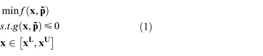
where the
It is difficult to obtain the accurate distribution of uncertainty in the practical engineering design. The uncertainties in this article are quantified by a series of intervals, namely, the uncertainty of a design scheme

where
We assume that an initial design scheme (

where the
A robust indicator of constraint is used to judge the feasibility of a design scheme. The inequality constraints of equation (1) can be rewritten as

Similarly, the variation of the equality constraint and objective function can be expressed as follows


The robustness of the objective function refers to how to determine the value of the design variables so that the variation of the objective function is as small as possible due to uncertainties. In practical engineering design, designers may not seek the most robust design of the objective function but require the objective function to be optimal within a prescribed range. Therefore, the objective function’s robustness index can be converted into constraints which are added to the original optimization problem. A robust design optimization model is given as follows
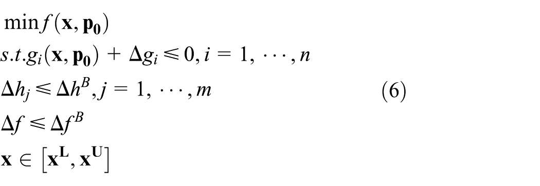
where f is the objective function, g is the vector of inequality constraints, and Δg, Δh, and Δf represent the maximum variation vector of inequality constraint, equality constraint, and the objective function, respectively. Δh
B
and Δf
B
are the bound values given by designers. The n denotes the number of inequality constraints and m denotes the number of equality constraints.

In the robust design of the objective function, if the goal is not to find the most robust solution of the objective function, it is necessary to prescribe the maximum variation bound of the objective function. However, Δh and Δf cannot be set arbitrarily. Because the values are set too large, it means that the equality constraints and the objective function can be in a large range of arbitrary fluctuations, so that the robust design will lose its original meaning. If the setting is too small, it is very likely that there is no solution, that is, in any solution design, solution of the equation variations or the objective function variations is greater than the set value, so it is extremely important to set a reasonable Δh and Δf. For the sake of expression, the changes of all uncertainties in the following text are expressed in terms of
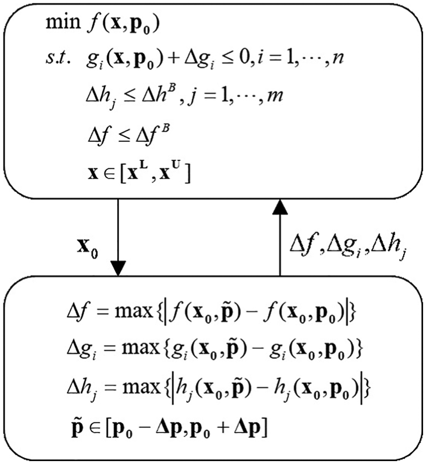
Robust design model under uncertainty.
MDO formulation
The general formulation of MDO problem is defined by
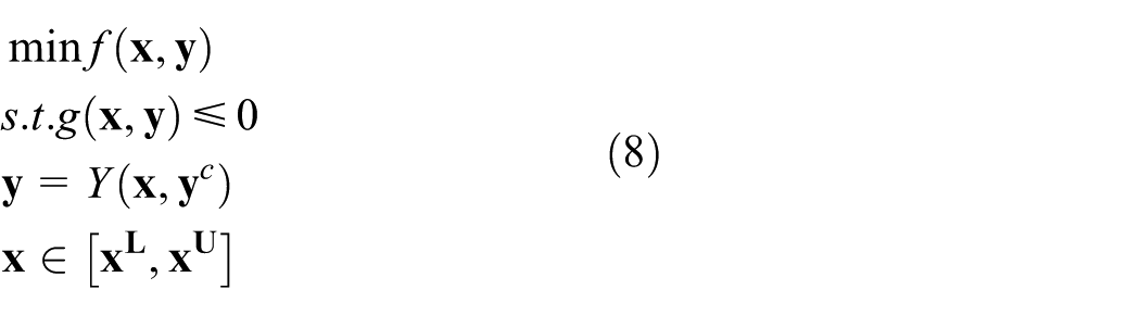
where g and f represent the constraints and the objective function of system, respectively. Y is the multidisciplinary analysis (MDA) function to obtain coupled state variable y.
Take a two-subsystem problem as an example (Figure 2).

MDO model of two subsystems.
Subsystems 1 and 2 are defined as follows


where gsub(i) and fsub(i) represent the constraints and objective function of ith subsystem, respectively. Ysub(i) denotes the analysis function associated with coupled state variable
Set strategy–based design optimization
To improve the efficiency of optimization, we adopt a set strategy to develop a novel MRDO method. The developed method is different from the previous MDO method, which can not only effectively decouple but also rapidly reduce the optimization search region and shorten the repetitive work of the optimization process. For ease of understanding, Figure 3 describes the difference between a point-based design and a set-based design.

Point-based design and set-based design.
Figure 3 illustrates boundary change of a simple design problem, with only two design variables. The light gray shade part of the figure shows the original design space. The left part of the figure describes the traditional point-based design. First, an initial point is given; then based on a gradient method, the search direction is constructed; or through an intelligent algorithm, a better solution is obtained. Finally, the optimal value of the objective function can be acquired by iterating sequentially. The right part of the figure shows the new design space, which is the smaller, purple shaded area. As described in “Introduction” section, one of the set-based design principles is to describe the design variables by changing the set of variables in the design process. The boundary between the design variables of the original MDO problem is defined in equation (8). Since the boundaries of design variables are getting smaller in the optimization process, this manner gives designers a way to decide. The purpose of the new MDO algorithm is to use a set-based approach to design and motivate design optimization. This means the design space is changed through the optimization process. In this way, we can avoid repeated analysis work and get the best design space. The results provide designers with the direction for subsequent analysis and decision making.
If a multidisciplinary system includes N subsystems, the objective functions of these subsystems may vary in order of magnitude. In addition, some target functions may vary greatly in the overall design space, while other changes are less. Therefore, the evaluation and comparison of different objective functions are contained. At first, those objective functions need to be normalized.
The main steps to reduce the design space are as follows:
First, normalize objective function value of subsystems.
The objective function values of subsystem i are normalized as follows

where
After normalization, we can find that the values of
Second, define and calculate subsystem space reduction rate.
Due to the complex coupling of MDO, a series of attempts have been made to reduce the search space. A simple and easy to calculate method is given. For instance, in the first cycle, for subsystem i, subsystem space reduction rate is defined and calculated by

where
Third, define and calculate system space reduction rate.
To ensure the accuracy of the solution, we should ensure that the search region contains the optimal solution. System space reduction rate is defined and calculated by

Finally, get new reduced design space.
The new search space in system level optimization is


The developed method
In this section, the developed approach is introduced thoroughly. First, after initial setting, a robust design is obtained for each subsystem. Second, the set strategy is utilized to search the robust space and solve the coupling variables during the optimization. Finally, the detailed steps and the head flowchart of the presented method are given.
MRDO under uncertainty
A complex mechanical system consists of different subsystems. Each subsystem has a specific function. Coupled relationships exist between different subsystems, which makes it difficult to evaluate the effect of uncertainties. The uncertainties of one subsystem not only affect its own subsystem but also affect other subsystems due to the relationships between these subsystems. This leads to the difficulty of solving multidisciplinary problems under uncertainty. This article develops a MRDO method by using a set-based strategy. The specific steps (take a two-subsystems as an example) are detailed below.
The following optimization framework is established for subsystem 1 considering variation of objective function, constraint condition, and the coupling state variable
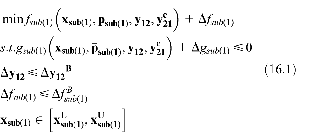
where

where
A similar structure for subsystem 2 is established in equation (17) and the same optimization strategy can be adopted

where

The system-level optimization is to coordinate the coupling variables from the full autonomy subsystems optimization. The system stage optimization model is given in equation (18). Furthermore, a two-level optimization model framework is developed, and the MRDO model can be established in Figure 4

where fsys() represents the objective function of system. Several strategies can be used to handle equation (18), for instance, MDF, IDF, SAND, ATC, and so on. In this article, we use the SAND29,30 strategy to address multidisciplinary coupling problem. The main advantage of SAND method is that it does not require a lot of system analysis and iterative process, which reduces the computational cost. The subsystem does not carry out systems analysis (SA) and subsystem optimization, and only calculates the maximum variation and value of the current point, then returns to system objective function.

The flowchart of MRDO.
Set strategy MDO procedure
In order to coordinate the coupling between subsystems, the improvement of system-level optimization model is as follows

where the fN represents the effect of the subsystem objective function, which is designed to make each subsystem relatively small. The closer the system is to the solution of the subsystem, the closer fN is to zero. Therefore, to minimize fN is to minimize the objective function of the subsystem. The fψ is to narrow the size of the design space as much as possible.
The steps and flowchart of the proposed method
We now summarize the implementation procedure of set-based MRDO. The stopping criteria of set-based MRDO method are as follows. (1) The objective approaches stability: the convergence error of the objective function between two consecutive cycles is less than a given value ε. (2) The cycle times exceed the maximum cycle, which means that the solution fails.
Main steps of proposed method are given as follows:
Step 1: Give initial points and bounds:
Step 2: Set
Step 3: Calculate all subsystem maximum
Step 4: Full autonomy is given to each subsystem to obtain robust optimal solution,
Step 5: According to
Step 6: In order to search the optimal solution as much as possible, we need to obtain the maximum
Step 7: Let the initial point of system stage optimization be
Step 8: According to
Step 9: Let cycle = cycle + 1, implement next iteration.
Step 10: If the cycle < Maxcycle, and the convergence error ≥ ε (convergence error = abs
Step 11: Otherwise, terminate the cycle process, output current optimal value.
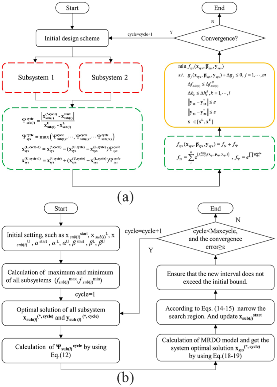
(a) The architecture of set-based MRDO and (b) the flowchart of set-based MRDO.
Based on the above discussions, for a two-subsystems MRDO problem, the architecture of set-based MRDO is shown in Figure 5(a) and a simplified flowchart of set-based MRDO is given in Figure 5(b).
Tests and results
In this section, two numerical examples and a speed reducer design problem are adopted to verify the accuracy and applicability of the developed approach. In addition, an air cooling battery thermal management system (BTMS) design problem is successfully solved by the proposed method. This means that the proposed method is the ability for addressing the practical engineering problem.
Test 1: Mathematical example 1
First, a simple math example was tested. The structure of problem is given in Figure 6. The simple problem was defined with only two design variables so that the results of the proposed method can easily be visualized in a two-dimensional plot. The two design variables are the x1 and the x2. The initial interval of x1 is [–5, 5] and x2 is [0, 6]. There are two subsystems: fsub(1) and fsub(2). Details for the mathematical model are provided as follows

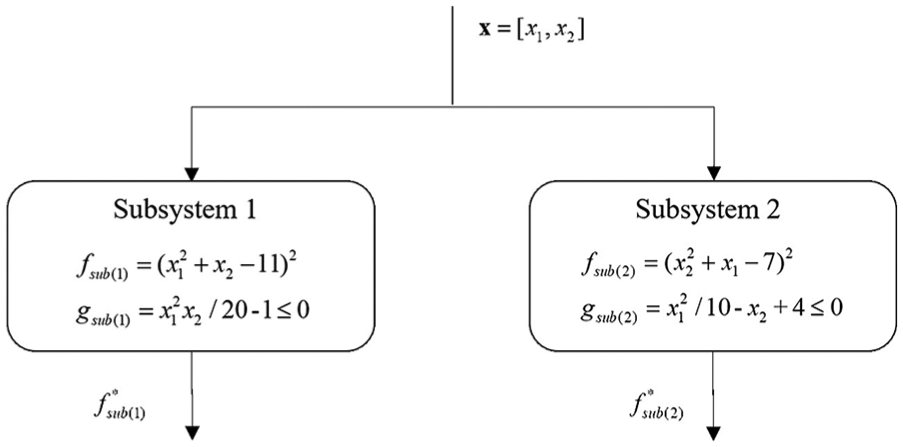
The structure of math example 1.
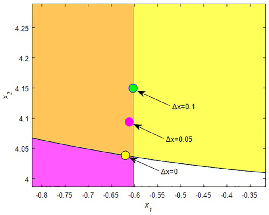
In this problem, the initial design point is [0,0]. We assume an uncontrollable variation in design variables x1 and x2. The two cases are calculated separately. The variations of
Optimization results.


The optimal solution of test 1 in individual subsystem.
The optimal solution of the individual subsystem 2.
The convergence error of optimization model.
In order to demonstrate the accuracy of the proposed method, a multilevel coordinate search (MCS) method using uniform distribution disordering the variation over the tolerance region was employed. Two cases’ robust optimal designs were used to verify the verification for the constraint robustness. The comparisons of constraint function robustness are shown in Figure 10 (1000 points are shown). In Figure 10, when there are uncertainties, the constraint conditions that the robust design is feasible and the nominal design scheme is hard to meet the design requirements.
The comparisons of constraint function robustness for g1 and g2.
We defined the reduction ratio of design region ψ as follows
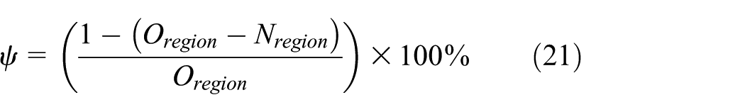
For Case 3, the ψ = (1 – 8.215 / 60) × 100% = 86.31%. The design space has been reduced by more than 86%, which provides more valuable information for the designer’s subsequent analysis and decision. In addition, if it is smaller than new design region, then the optimal solution of the subsystem will not be included, and then the key information will be lost.
Test 2: Mathematical example 2
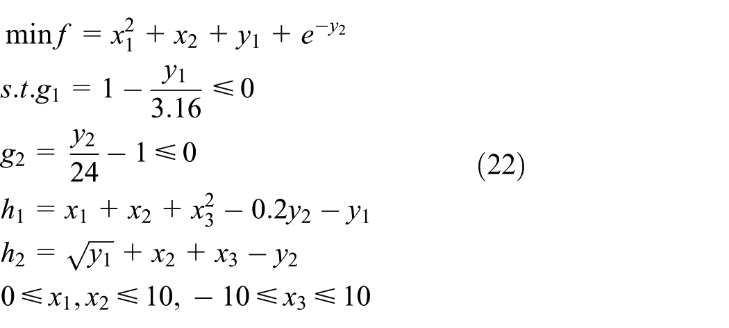
A classic MDO problem including two disciplines was used for verification. 28 Each discipline has a coupled state variable; nonlinear coupled relationship exists between two subsystems (Figure 11). The optimization model is expressed as follows

The MDO model of math problem 2.
To illustrate this question more intuitively, we divide the problem into two subsystems, as shown in the Figure 11. The variations of
Optimization results.


The optimal solution of two cases in individual subsystem.
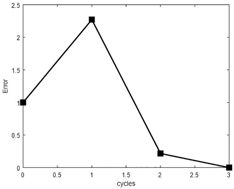
The convergence error of optimization model.

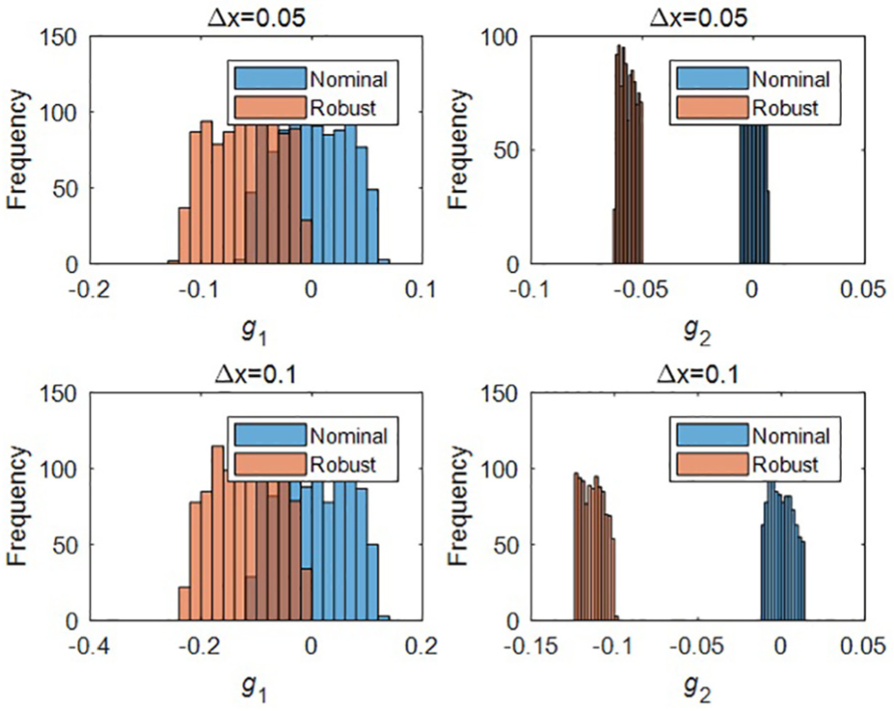
The comparisons of constraint function robustness for g1 and g2.
In Table 2, the “Origin” row describes the initial lower and upper bounds of design variables. The “New” row describes the design results using the proposed method. Due to the existence of the coupled state variables, we cannot obtain the optimal solution of subsystem in individual optimization. The new boundaries for the design space are shown as light green cube, and the subsystem optima within the new design space are shown as pink markers. In this problem, the ψ = (1 – 650.86 / 2000) × 100% = 67.46%. The design region has been reduced by more than 67%, that is, this method can greatly decrease the rework and reanalysis. It has broad prospects for comprehensive design of complex systems.
Test 3: The speed reducer design
The speed reducer design problem is a standard MDO test. 45 Figure 15 illustrates the speed reducer diagram. The design objective is to minimize the volume of the structure (objective function). The main constrains are the bending stress and contact stress of the gear tooth, the torsional deformation, and stress requirements of the shaft


where x1 is gear tooth width, x2 is the teeth module, x3 is the number of teeth of the pinion, x4 is the distance between the bearing 1, x5 is the distance between bearing 2, x6 is the diameter of the shaft 1, x7 is the diameter of the shaft 2, g1 and g2 are constraints of gear tooth bending stress and contact stress, g3∼g8 are constraints of the shaft deformation, stress, and g9∼g11 are geometric constraints. Assume that the x2 and x6 have interval uncertainty (Δx2, Δx6) = (0.01, 0.1). We divide the reducer design model into three subsystems, namely, subsystem 1 (gear), subsystem 2 (shaft 1), and subsystem 3 (shaft 2), respectively (Figure 16). The acceptable objective variation range of

The structural diagram of speed reducer.

The MDO model of speed reducer.
For robust design, the optimal robust solution for subsystem 1 is
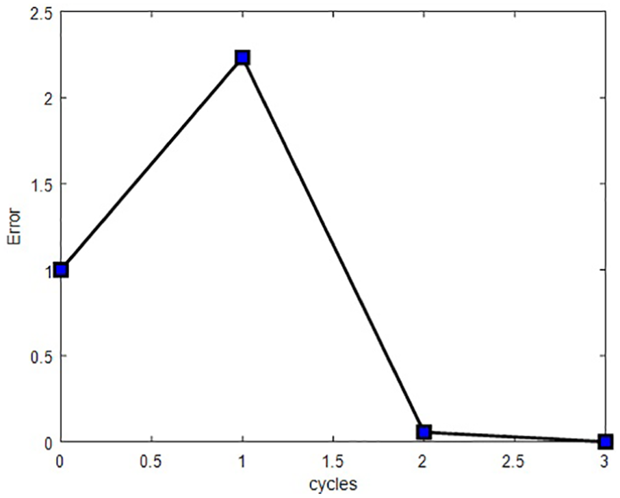
The results are shown in Table 3. For Case 2, the calculation times of Sys, Sub 1, Sub 2, and Sub 3 are 3025, 391, 731, and 46, correspondingly. The convergence error of the system-level cycle is shown in Figure 17. It also only takes three cycles to get the optimal which is the accuracy and efficiency of the proposed method. The “O” row gives the initial bounds of design variables. The “N” row represents the design results using the proposed method. Because there are more than three design variables, we cannot be intuitive to see the design space changes. So the “Δ” row describes the reduction ratio of each design variables (by equation (21)). It is can be seen from the “Δ” row that every design variables have been reduced by more than 87% except x2 and x3. The biggest of the multidisciplinary compromise is in f2 (robust design solution is 9% more than nominal design). The system optima for f1 and f3 are relatively close to the subsystem optimal solution. As similar to the discussion in “Test 1: Mathematical example 1” and “Test 2: Mathematical example 2” sections, MCS method is applied. The nominal design and robust design were used to verify the confirmation for the constraint robustness. There are no uncertainties in subsystem 3, so we do not analyze the constraints of g4, g6, and g11. The comparisons of constraint function robustness are shown in Table 4 and Figure 18 (1000 points are shown). In Figure 17, when there are uncertainties, the constraint conditions that the robust design is feasible and the nominal design scheme for g5 and g8 is difficult to meet the design requirements.
Optimization results (unit: mm).

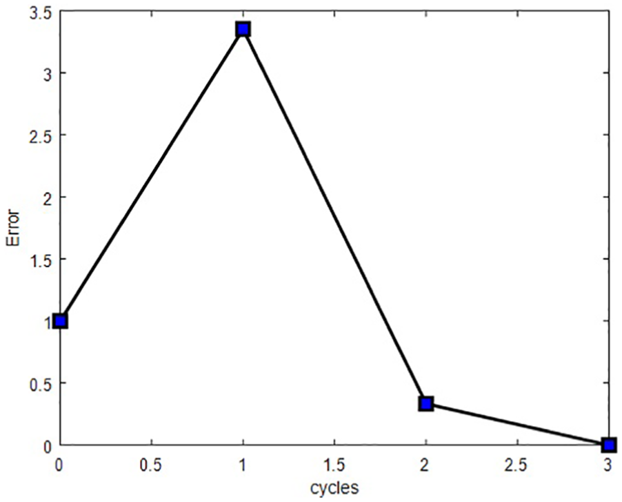
The convergence error of optimization model for speed reducer.
The probability of constraint function robustness for subsystem 2 and subsystem 3.

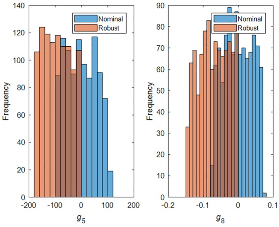
The comparisons of constraint function robustness for g5 and g8.
Test 4: Air cooling BTMS design
An air-cooled module containing eight cells had been well defined by National Renewable Energy Laboratory in their previous work. 46 It is discharged and charged under normal driving conditions. Air cooling BTMS design involves five design variables that are d1, d2, d3, d4, and v. Schematic diagram of the battery module is shown in Figure 19. More details can be seen in Fan et al. 46 and Li et al. 47

Schematic diagram of the battery module.
Some notations are defined in this work. TD is the maximum temperature difference of eight cells (calculated by mean temperature) and TSD is the temperature standard deviation. Computational domain of the battery module with air cooling is shown in Figure 20.

Computational domain of the battery module with air cooling.
Without loss of generality, the mathematical model of multidisciplinary optimization is given with all-in-one formulation as follows

In this article, to reduce the cost of the expensive computational fluid dynamics (CFD) process and have high approximation accuracy, Kriging model is applied for surrogate model and built similar to Li et al. 47 and Stein. 48 The maximum temperature difference and temperature standard deviation surrogate models are represented by equations (25 and 26)


In this work, the air cooling battery module is analyzed in ANSYS by incorporating the basic information as mentioned in Zhang et al.
49
In this example, large weight is assigned to the battery temperature difference. The design variables x with Δ
Optimization results of air cooling BTMS.

BTMS: battery thermal management system.

Temperature distributions (unit: K) within the cells for the (a) initial scheme of battery module, (b) nominal optimum of battery module, and (c) robust optimum of battery module.
MCS method is applied to verify the accuracy of the developed method. The comparisons of constraint function robustness for g1 and g2 are presented in Figure 22. Only 50 points are shown, since the simulation is time-consuming. Note that this operation does not change the nature of the problem. In Figure 22, when there are no uncertainties, the nominal design scheme and the robust design scheme for g1 are both feasible. However, in Figure 22, when there are uncertainties, the constraint conditions that the robust design is still feasible and the nominal design scheme for g2 is hard to meet the design requirements.

The comparisons of constraint function robustness for g1 and g2.
Conclusion
Coupled relationships exist between different subsystems, which makes it difficult to evaluate the effect of uncertainties. The uncertainties of one subsystem not only affect its own subsystem but also affect other subsystems due to the relationships between these subsystems. This leads to the difficulty of solving multidisciplinary problems under uncertainty. In this article, first, two design methodologies based on point design and set design are compared. Then, a two-level optimization model framework is developed; the lower level is to obtain the optimal robust solution for each subsystem by adopting full autonomy optimization and the system-level optimization is to coordinate the coupling variables from the full autonomy subsystem optimization. Furthermore, we make a try to integrate the set strategy into the MRDO method. Finally, two mathematics examples and the speed reducer design problem verify the validity and accuracy of the proposed method. A practical engineering problem, namely air cooling BTMS design problem, is successfully solved by the proposed method. This means that the proposed method is the ability for addressing the practical engineering problem.
Moreover, the main advantages of the developed method can be summarized as follows. (1) It can effectively coordinate all subsystems and get the global optimal. (2) It obviously narrows the design space and provides feasible direction for the designer’s subsequent design and decision. (3) It is relatively simple and easy to be implemented and the solving process is accurate and stable.
In addition, although a set-based design found many merits for complex systems, it has a lot of work to be done, for instance, if there are time-varying uncertainties in the system. As part of future work, the developed method with surrogate model should be developed.
Footnotes
Handling Editor: José Correia
Declaration of conflicting interests
The author(s) declared no potential conflicts of interest with respect to the research, authorship, and/or publication of this article.
Funding
The author(s) disclosed receipt of the following financial support for the research, authorship, and/or publication of this article: This work was supported by the National Natural Science Foundation of China (grant numbers 51675196 and 51721092) and the Program for HUST Academic Frontier Youth Team.